R basics
Getting used to R
Franziska Faupel
MOSAIC Summer School 2016
Structure
- First Part
- Vectors
- Functions
- Operators
- Data Frames, Matrices & Arrays
- Second Part
- Load data
- Manipulate Data
- Loops and Restrictions
- Loading Packages
- Plots

1. Load Data
1. Load Data | Where is your project at home?
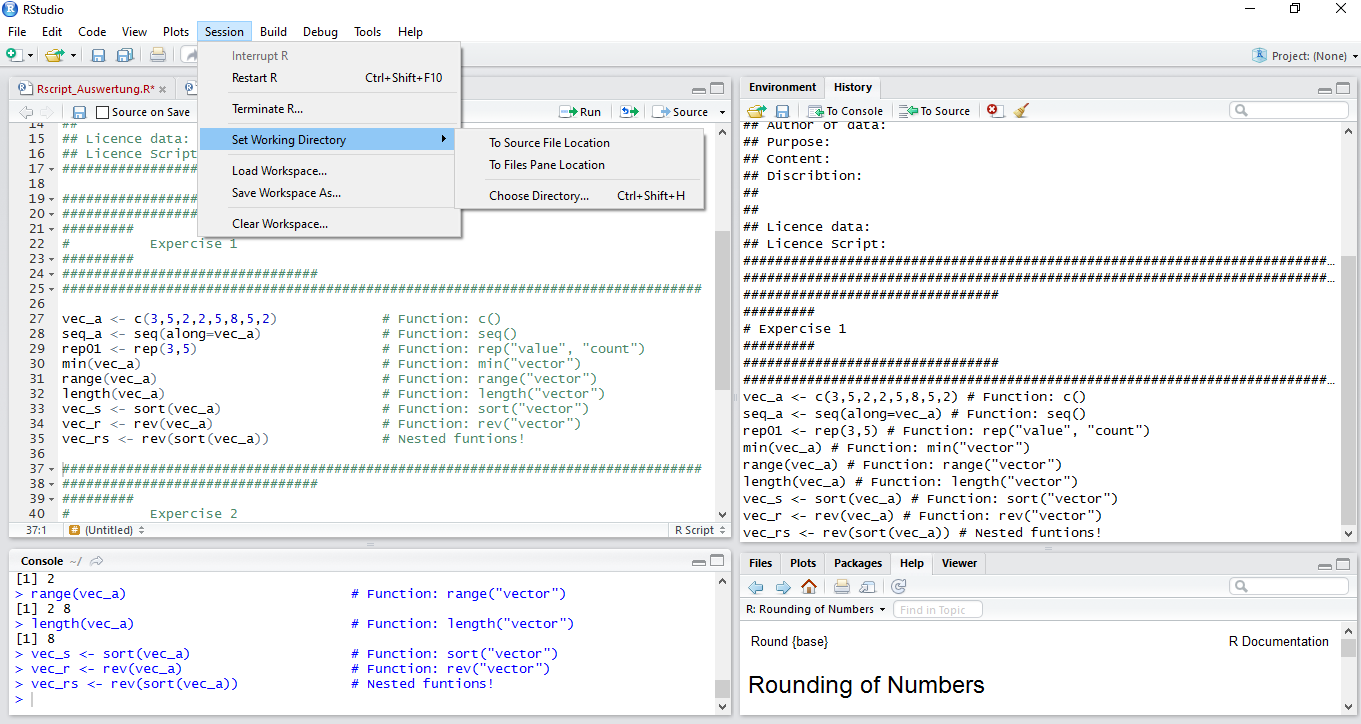
1. Load Data | Where is your project at home?
wd <- "C:\\Folder\\Subfolder\\SubSubFolder"
setwd(wd)

wd <- "/home/xxx/subFolder/SubSubFolder"
setwd(wd)
1. Load Data | Loading a Data Table
df_mounds <- read.table('gravemounds.csv', header=TRUE, sep=';')
# See ?read.table for further information

filename <- "gravemounds02.csv" # Creating a string vector

# Writing a data frame
write.table(df_mounds, file = filename, quote = FALSE,
sep = ";", na = "NA", dec = ".", row.names = TRUE, col.names = TRUE)
1. Load Data | Loading a Data Table
df_mounds
##                    Nekropole Gravemounds Inhumation Incremation Epoche
## 1            Schelmenhostadt           8          y           y   both
## 2                  Heuschier           6                            BA
## 3                Wolfswinkel          33          y           y   both
## 4                  Deilsberg          14                      y     BA
## 5               Taubenhuebel          12          y           y   both
## 6                   Eichlach          16          y           y     BA
## 7                 Fischereck           7          y           y   both
## 8             Hatternstangen          18                      y     BA
## 9        Dachhuebel-Birklach          20          y           y     BA
## 10                Beckenmatt          31          y                 BA
## 11        Weisensee-Oberfeld          63          y           y   both
## 12                   Erzlach           5                            BA
## 13                 Donauberg          14          y           y   both
## 14               Koenigsberg          23          y           y   both
## 15 Fischerhuebel-Kurzgelaend          98          y           y   both
## 16           Schirrheinerweg          17          y           y   both
## 17                 Kirchlach         120          y           y   both
## 18                     Gries           5                          both
## 19                 Weitbruch          15          y           y     BA
## 20                 Harthouse          15          y           y   both
## 21                  Maegstub          31                          both
## 22              Oberstritten           1                            BA
## 23                  Ohlungen           3                      y     IA
## 24                 Uhlwiller          15                      y     IA
##    Excavated     Literature Bronze Ceramics Amber Gold Glass Iron Stone
## 1          8 Schaeffer 1926     43        8     9   NA     1    1     1
## 2          1 Schaeffer 1926     NA       NA    NA   NA    NA   NA    NA
## 3         12 Schaeffer 1930     13        9    NA   NA    NA   NA    NA
## 4          5 Schaeffer 1926     12        3     3    1     2   NA    NA
## 5          7 Schaeffer 1930     29        9     1   NA    NA   NA    NA
## 6          9 Schaeffer 1926      7        9    NA   NA    NA   NA     1
## 7          7 Schaeffer 1930     14        4    NA   NA    NA   NA     2
## 8          9 Schaeffer 1926      4       11    NA   NA    NA   NA    NA
## 9          7 Schaeffer 1926     23       13     4   NA    NA   NA    NA
## 10        26 Schaeffer 1926     15       24    NA   NA    NA   NA    NA
## 11        38 Schaeffer 1930     88       62     8    1    NA    5    NA
## 12         5 Schaeffer 1926      3       NA    NA   NA    NA   NA    NA
## 13        14 Schaeffer 1930     68       24    NA   NA     1    2    NA
## 14        20 Schaeffer 1930    257       50     7    3    11   30     6
## 15        89 Schaeffer 1930    304       90    20    2     8   19    13
## 16        13 Schaeffer 1930     62       11    NA    2     1    3     4
## 17       100 Schaeffer 1930    134      173    12   NA     3   13     4
## 18         2 Schaeffer 1930      7       18    NA   NA    NA   NA    NA
## 19         7 Schaeffer 1930     53       11    NA    2    NA    5    NA
## 20         9 Schaeffer 1930    118       19    NA   NA     2   10    16
## 21        13 Schaeffer 1930    309       23    10    3    10   31     9
## 22         1 Schaeffer 1926      8        1    NA   NA    NA   NA    NA
## 23         3 Schaeffer 1930    101       NA    12    4    16    3    12
## 24        14 Schaeffer 1930     49        1     1   NA     3    9     1
##    Coral       X       Y
## 1     NA 3419142 5416936
## 2     NA 3417717 5415907
## 3     NA 3421495 5415052
## 4     NA 3423415 5413753
## 5     NA 3419884 5414973
## 6     NA 3419139 5413198
## 7     NA 3416267 5413553
## 8     NA 3417327 5412854
## 9     NA 3412431 5412258
## 10    NA 3419640 5411492
## 11    NA 3422261 5411072
## 12    NA 3423314 5411595
## 13    NA 3424722 5411495
## 14     2 3425604 5412985
## 15     3 3422962 5409879
## 16     1 3421628 5408831
## 17    NA 3419741 5408021
## 18    NA 3412957 5404536
## 19    NA 3411268 5404405
## 20     1 3406774 5406406
## 21     1 3406705 5411437
## 22    NA 3412351 5418083
## 23     3 3405413 5410742
## 24    NA 3404224 5411166
1. Load Data | Creating new Data Frames using subset
df_BA <- subset(df_mounds, df_mounds$Epoche == "BA")
df_BA_INH <- subset(df_mounds, df_mounds$Epoche == "BA" & df_mounds$Inhumation == "y")
str(df_BA_INH)
## 'data.frame':    4 obs. of  17 variables:
##  $ Nekropole  : Factor w/ 24 levels "Beckenmatt","Dachhuebel-Birklach",..: 5 2 1 23
##  $ Gravemounds: int  16 20 31 15
##  $ Inhumation : Factor w/ 2 levels "","y": 2 2 2 2
##  $ Incremation: Factor w/ 2 levels "","y": 2 2 1 2
##  $ Epoche     : Factor w/ 3 levels "BA","both","IA": 1 1 1 1
##  $ Excavated  : int  9 7 26 7
##  $ Literature : Factor w/ 2 levels "Schaeffer 1926",..: 1 1 1 2
##  $ Bronze     : int  7 23 15 53
##  $ Ceramics   : int  9 13 24 11
##  $ Amber      : int  NA 4 NA NA
##  $ Gold       : int  NA NA NA 2
##  $ Glass      : int  NA NA NA NA
##  $ Iron       : int  NA NA NA 5
##  $ Stone      : int  1 NA NA NA
##  $ Coral      : int  NA NA NA NA
##  $ X          : num  3419139 3412431 3419640 3411268
##  $ Y          : num  5413198 5412258 5411492 5404405
1. Load Data | Save your current environement

1. Load Data | Save your current environement
save.image("7ws/name01.rws")
load("7ws/name01.rws")
2. Manipulate Data
2. Manipulate Data | How to choose a specific value
df <- df_mounds # Coping df_mounds
df[c(1:3),c(2,3)]
##   Gravemounds Inhumation
## 1           8          y
## 2           6
## 3          33          y
df[3, c(1,3)]
##     Nekropole Inhumation
## 3 Wolfswinkel          y
... and to change it
df[c(6,7,8),3] <- NA # Asign these values with NA
df[c(6,7,8),3]
## [1] <NA> <NA> <NA>
## Levels:  y
2. Manipulate Data | How to choose a specific value
vector[...]
df[ row , col ]
| argument | effect | Example |
|---|---|---|
| positive integer | returns specified elements | c(1,3:4) or 2 |
| negative integer | returns all other elements | c(-1,-3:4) or -2 |
| blank spaces | returns all | |
| names | return those with specific names | c("name", "type") or "name" |
| logical | returns elements, that corresponds to TRUE | c(TRUE, FALSE) or TRUE |
2. Manipulate Data | Adding new Columns
df$newcol <- df$Excavated/df$Gravemounds*100
df$newcol
##  [1] 100.00000  16.66667  36.36364  35.71429  58.33333  56.25000 100.00000
##  [8]  50.00000  35.00000  83.87097  60.31746 100.00000 100.00000  86.95652
## [15]  90.81633  76.47059  83.33333  40.00000  46.66667  60.00000  41.93548
## [22] 100.00000 100.00000  93.33333
2. Manipulate Data | Combine Data Frames
merge(x, y, by = intersect(names(x), names(y)),
      by.x = by, by.y = by, all = FALSE, all.x = all, all.y = all,
      sort = TRUE, suffixes = c(".x",".y"),
      incomparables = NULL, ...)
2. Manipulate Data | Merge Data Frames
ndf<- merge(df_mounds, df, all.x=TRUE, all.y=FALSE, by.x="Nekropole",
                    by.y="Nekropole")
2. Manipulate Data | Combine Data Frames
str(ndf)
## 'data.frame':    24 obs. of  34 variables:
##  $ Nekropole    : Factor w/ 24 levels "Beckenmatt","Dachhuebel-Birklach",..: 1 2 3 4 5 6 7 8 9 10 ...
##  $ Gravemounds.x: int  31 20 14 14 16 5 7 98 5 15 ...
##  $ Inhumation.x : Factor w/ 2 levels "","y": 2 2 1 2 2 1 2 2 1 2 ...
##  $ Incremation.x: Factor w/ 2 levels "","y": 1 2 2 2 2 1 2 2 1 2 ...
##  $ Epoche.x     : Factor w/ 3 levels "BA","both","IA": 1 1 1 2 1 1 2 2 2 2 ...
##  $ Excavated.x  : int  26 7 5 14 9 5 7 89 2 9 ...
##  $ Literature.x : Factor w/ 2 levels "Schaeffer 1926",..: 1 1 1 2 1 1 2 2 2 2 ...
##  $ Bronze.x     : int  15 23 12 68 7 3 14 304 7 118 ...
##  $ Ceramics.x   : int  24 13 3 24 9 NA 4 90 18 19 ...
##  $ Amber.x      : int  NA 4 3 NA NA NA NA 20 NA NA ...
##  $ Gold.x       : int  NA NA 1 NA NA NA NA 2 NA NA ...
##  $ Glass.x      : int  NA NA 2 1 NA NA NA 8 NA 2 ...
##  $ Iron.x       : int  NA NA NA 2 NA NA NA 19 NA 10 ...
##  $ Stone.x      : int  NA NA NA NA 1 NA 2 13 NA 16 ...
##  $ Coral.x      : int  NA NA NA NA NA NA NA 3 NA 1 ...
##  $ X.x          : num  3419640 3412431 3423415 3424722 3419139 ...
##  $ Y.x          : num  5411492 5412258 5413753 5411495 5413198 ...
##  $ Gravemounds.y: int  31 20 14 14 16 5 7 98 5 15 ...
##  $ Inhumation.y : Factor w/ 2 levels "","y": 2 2 1 2 NA 1 NA 2 1 2 ...
##  $ Incremation.y: Factor w/ 2 levels "","y": 1 2 2 2 2 1 2 2 1 2 ...
##  $ Epoche.y     : Factor w/ 3 levels "BA","both","IA": 1 1 1 2 1 1 2 2 2 2 ...
##  $ Excavated.y  : int  26 7 5 14 9 5 7 89 2 9 ...
##  $ Literature.y : Factor w/ 2 levels "Schaeffer 1926",..: 1 1 1 2 1 1 2 2 2 2 ...
##  $ Bronze.y     : int  15 23 12 68 7 3 14 304 7 118 ...
##  $ Ceramics.y   : int  24 13 3 24 9 NA 4 90 18 19 ...
##  $ Amber.y      : int  NA 4 3 NA NA NA NA 20 NA NA ...
##  $ Gold.y       : int  NA NA 1 NA NA NA NA 2 NA NA ...
##  $ Glass.y      : int  NA NA 2 1 NA NA NA 8 NA 2 ...
##  $ Iron.y       : int  NA NA NA 2 NA NA NA 19 NA 10 ...
##  $ Stone.y      : int  NA NA NA NA 1 NA 2 13 NA 16 ...
##  $ Coral.y      : int  NA NA NA NA NA NA NA 3 NA 1 ...
##  $ X.y          : num  3419640 3412431 3423415 3424722 3419139 ...
##  $ Y.y          : num  5411492 5412258 5413753 5411495 5413198 ...
##  $ newcol       : num  83.9 35 35.7 100 56.2 ...
2. Manipulate Data | Combine Data Frames
cbind(x,y) # Combines data frames columnwise
rbind(x,y) # Combines data frames rowise
2. Manipulate Data | Unique
unique(x, incomparables = FALSE, fromLast = FALSE, ...)
... unique() returns a vector, data frame or array like x but with duplicate elements/rows removed.
df <- data.frame(V1 = c(1,1,1), V2 = c(2,2,2), V3 = c("A","A","B"))
unique(df)
##   V1 V2 V3
## 1  1  2  A
## 3  1  2  B
uni_v3 <- unique(df$V3)
uni_v3
## [1] A B
## Levels: A B
2. Manipulate Data | Unique
duplicated(x, incomparables = FALSE, fromLast = FALSE, nmax = NA, ...)
... duplicated() determines which elements of a vector or data frame are duplicates of elements with smaller subscripts, and returns a logical vector indicating which elements (rows) are duplicates.
df
##   V1 V2 V3
## 1  1  2  A
## 2  1  2  A
## 3  1  2  B
duplicated(x = df, fromLast = TRUE)
## [1]  TRUE FALSE FALSE
3. Loops and Restrictions
3. Loops and Restrictions
Loops repeat statements
# Loops repeat statements
a <- 1
for (i in 1:20){
a <- a+a
}
3. Loops and Restrictions
Loops repeat statements
# Loops repeat statements
a <- 1
for (i in 1:20){
a <- a+a
}

a
## [1] 1048576
3. Loops and Restrictions
# conditions restrict statements
i <- 1
a <- 1

while (a <55){
a <-a+a
i=i+1
}
3. Loops and Restrictions
# conditions restrict statements
i <- 1
a <- 1

while (a <55){
a <-a+a
i=i+1
}

a
## [1] 64
i
## [1] 7
3. Loops and Restrictions
# conditions restrict statements
if (a>55){
a <- a/2
} else {
a <- a*2
}
3. Loops and Restrictions
# conditions restrict statements
a
## [1] 32

if (a>55){
a <- a/2
} else {
a <- a*2
}
a
## [1] 64
3. Loops and Restrictions
| Loops or Restrictions | starts | Condistions | Indside | Ends |
|---|---|---|---|---|
| Loop | for |
(i in "repetition") |
{ result <- "functions to apply" |
} in a seperate line |
| Restrictions | while |
(i in "condition") |
{ result <- "functions to apply" |
} in a seperate line |
| Restrictions | if in combination with else |
(i in "condition") |
{ result <- "functions to apply" |
} in a seperate line |
| Restrictions | else |
(i in "condition") |
{ result <- "functions to apply" |
} in a seperate line |
4. Package management
4. Package management
Package management:
old.packages()                        # Your currently installed packages

update.packages()                     # Update all Packages
update.packages("package-name")       # Update a specific package
Loading Packages:
install.packages("package-name") # Download and install the named package
Using Packages:
library(package-name) # Loading packages every time you restart R!
5. Plots
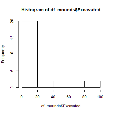
5. Plots | Histogram
hist_gm <- hist(df_mounds$Gravemounds)
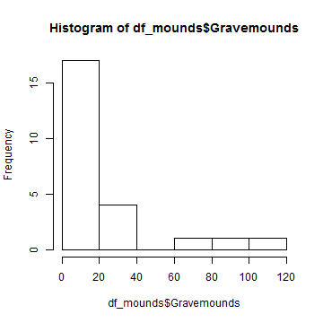
hist_ex <- hist(df_mounds$Excavated)
5. Plots | Histogram
plot(hist_gm, main="Gravemounds of Haguenau Froest", xlab="Number of Gravemounds",
     sub="Schaeffer 1926/1930", col="dark red")

Plots | Violinplots
library(vioplot)
vioplot(df_mounds$Gravemounds)

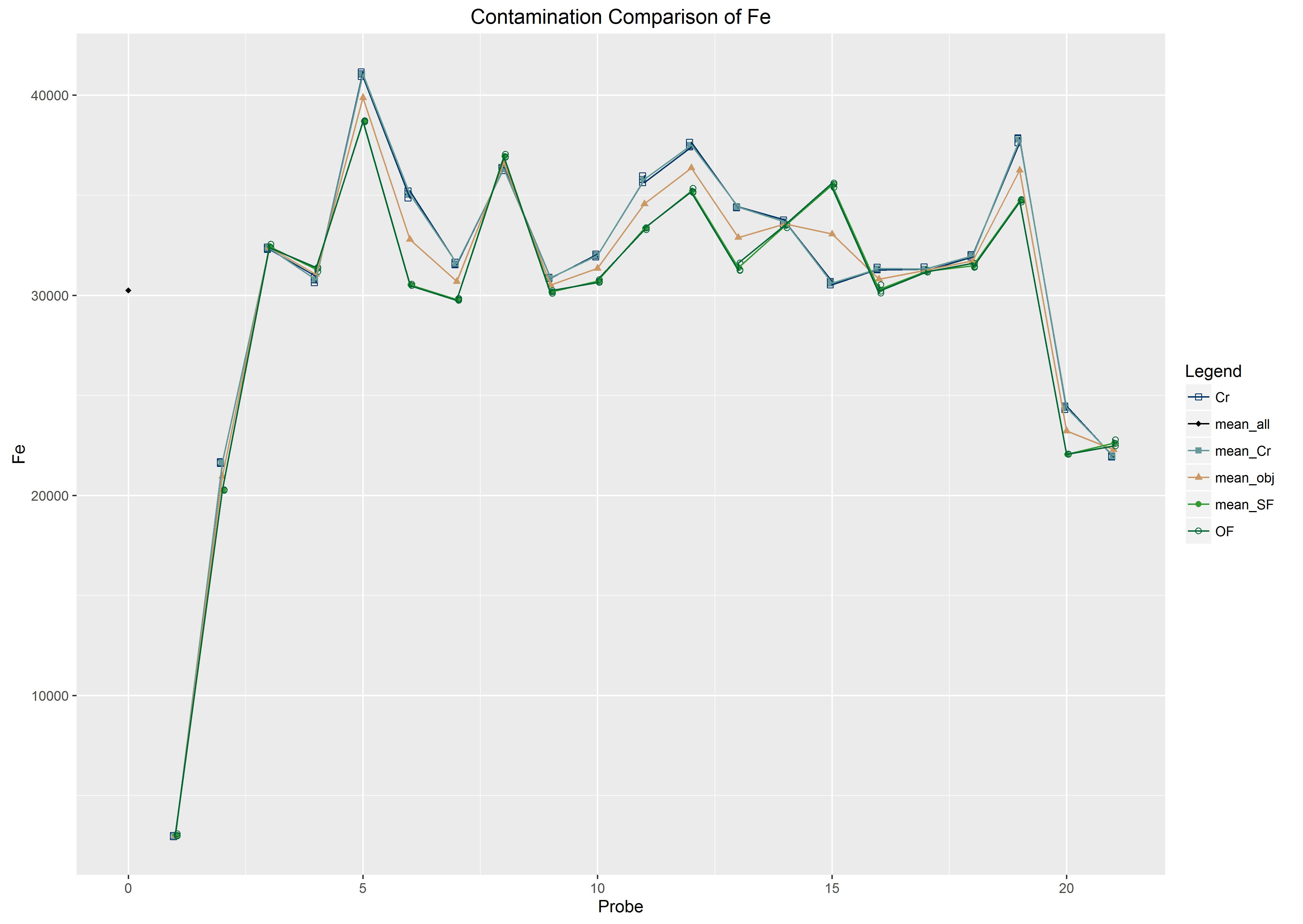
Plots | ggplot2
library(ggplot2)
Exercise 3
# 1. Set your working directory.
# 2. Load gravemound.csv
# 3. Save created Data Frame of Iron Age graves using `subset`
# 4. Save this Data Frame in your Subfolder `2data`
# 5. Explore following functions `rbind()` and `cbind`
# 6. Create and edit a Histogramm and a Violinplot.
# 7. Use `?plot` to create a scatterplot.
# 8. Download and load all neccessary packages for our next lecture.
Presentations
Monday, 5th of September
Tuesday, 6th of September
Wednesday, 7th of September
- Modelling Interaction: Cultural & Geographic Distance
- Workshop: Geographical and Economic Distances
- Workshop: Cultural Distances
Thursday, 8th of September
- Modelling Interaction: Network Approaches
- Workshop: Pointpattern Analysis
- Workshop: Network Analysis