Introduction to baytaAAR • baytaAAR

Load libraries

library(baytaAAR)
library(ggplot2)
library(bayesplot)
library(tidybayes)
library(flexsurv)

Introduction

baytaAAR implements latent trait analysis within a Bayesian Markov Chain Monte Carlo (MCMC) framework. It is intended to estimate the age-of-death of adult individuals for whom one or several ordinal traits related to the human aging process have been assessed. It produces probability densities for the individual ages but also for the respective population as a whole. baytaAAR has been introduced and tested by Müller-Scheeßel et al. (2026), and there the basic idea of the model is illustrated in the following figure:

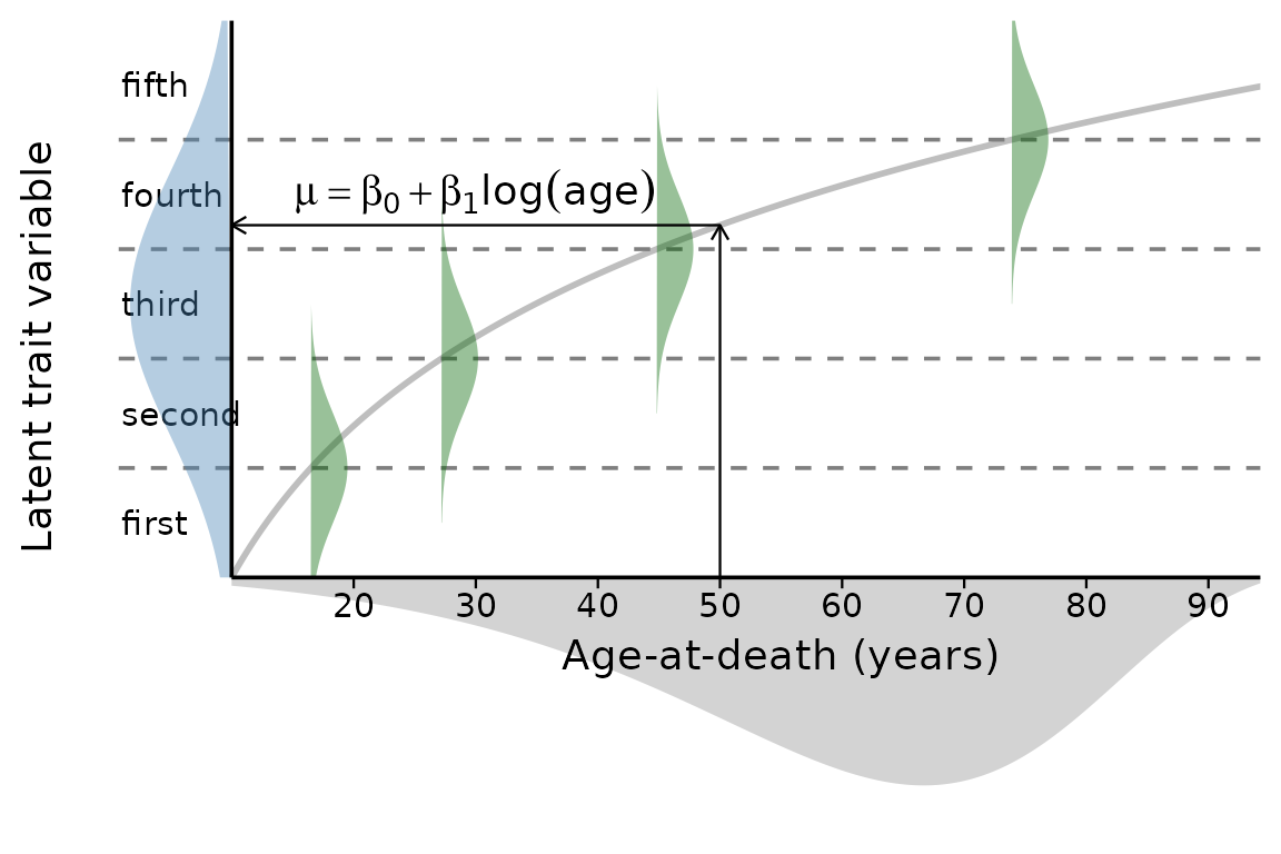
The figure schematically visualizes the ordered probit regression as a latent trait approach with age-at-death estimated from a Gompertz distribution (grey area). The green Gaussian distributions symbolize the transitions between the trait stages (here, arbitrarily, 5 stages, therefore 4 transitions). The regression line with its parameters intercept ( $\beta_0$ ) and slope ( $\beta_1$ ) determines the position of the latent trait variable. Please note that age is log-scaled, so the regression line appears curved. In practical applications, the latent trait variable does not need to be centered as it is here and the transitions are unlikely to be as evenly spaced as shown here.

More in-depth information on the background of and the rationale behind baytaAAR can be found in the vignettes. One of them discusses a real-life use-case with partly known ages-at-death.

Data layout

As input, the function bay.ta() assumes a matrix() of trait expressions. In its simplest form, this may contain only one column with a single trait as in the following example (“auricular surface”):

data(sorsum_as, package = "baytaAAR")
head(sorsum_as)
#>     id auricular_surface
#> 1  700                 4
#> 4  704                 5
#> 9  710                 8
#> 10 711                 4
#> 16 717                 6
#> 17 719                 3

The example stems from the neolithic gallery grave Sorsum in Hessen/Germany. The auricular surface was the trait which was possible to assess most often (data from Moser et al. 2025, table S69), and it was assessed according to the method by Lovejoy et al (1985) which comprises eight levels. An overview of the distribution of the levels is given in the following plot:

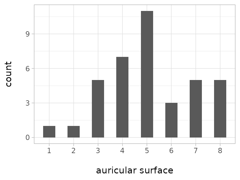
Level 5 is the most numerous while levels 1 and 2 are only present once each. More on data input can be found in the vignette("data_preparation").

Running a first analysis

We will now run a first analysis with bay.ta() with the Sorsum data. We will leave most parameters at the default values and only change the minimum age to 18 and the thinning interval (thinsteps) to 1000. This number is multiplied with the number of saved steps (1000) and the result divided by the number of chains (default = 3) to obtain the total number of iterations, minus the number of iterations used for burning-in. We also set a seed for reproducibility.

sorsum_as_res <- bay.ta(
  method = sorsum_as[,2],
  minimum_age = 18,
  thinSteps = 1000,
  numSavedSteps = 1000,
  seed = 1234
)
#> Starting Time: 31 May 2026 20:51:44
#> Defining model
#> Building model
#> Setting data and initial values
#> Running calculate on model
#>   [Note] Any error reports that follow may simply reflect missing values in model variables.
#> Checking model sizes and dimensions
#> Checking model calculations
#> Compiling
#>   [Note] This may take a minute.
#>   [Note] Use 'showCompilerOutput = TRUE' to see C++ compilation details.
#> ===== Monitors =====
#> thin = 1: a, age.s, b, beta, beta0, thresh
#> ===== Samplers =====
#> RW sampler (85)
#>   - age[]  (38 elements)
#>   - beta[]  (1 element)
#>   - beta0[]  (1 element)
#>   - b
#>   - thresh[]  (6 elements)
#>   - ystar[]  (38 elements)
#> Compiling
#>   [Note] This may take a minute.
#>   [Note] Use 'showCompilerOutput = TRUE' to see C++ compilation details.
#> running chain 1...
#> |-------------|-------------|-------------|-------------|
#> |-------------------------------------------------------|
#> running chain 2...
#> |-------------|-------------|-------------|-------------|
#> |-------------------------------------------------------|
#> running chain 3...
#> |-------------|-------------|-------------|-------------|
#> |-------------------------------------------------------|
#> Execution Time: 1.39 minutes

The analysis takes about 1 minute, depending on the computer power. The console output informs about the monitored parameters (a, age.s, b, beta, beta0, thresh), the sampled nodes (age, beta, beta0, b, thresh and ystar), their number and the used sampler which is RW for Metropolis-Hastings sampling. The model output (sorsum_as_res in this case) is a matrix with the number of chains (three in the default case).

The output can be processed with any function able to deal with coda::mcmc.lists() but baytaAAR provides some functions for convenience to quickly achieve diagnostic results. One of them is the function diagnostic.summary which does exactly what its name suggests: a summary of diagnostic measures of the parameters.

sorsum_as_res_diag <- diagnostic.summary(sorsum_as_res) 
sorsum_as_res_diag |> head(10) |> knitr::kable(digits = 4)

	PSRF Point est.	PSRF Upper C.I.	Mean	Median	Mode	ESS	MCSE	HDImass	HDIlow	HDIhigh
M	1.0235	1.0748	55.4075	60.1760	70.5845	620.9	0.7614	0.95	17.1554	81.7739
a	1.0226	1.0740	0.0091	0.0073	0.0029	621.7	0.0003	0.95	0.0002	0.0231
age.s[1]	1.0086	1.0309	45.1235	43.6152	40.7268	708.6	0.4788	0.95	20.8396	67.7356
age.s[2]	1.0041	1.0208	57.7845	57.2079	53.0281	666.3	0.5238	0.95	31.7521	81.9953
age.s[3]	1.0341	1.1155	82.9289	83.5910	82.9695	860.7	0.3295	0.95	65.2826	99.9182
age.s[4]	1.0123	1.0340	45.6070	44.4307	38.5401	647.7	0.5230	0.95	20.6297	70.8874
age.s[5]	1.0088	1.0322	67.1531	67.3303	72.0938	528.2	0.5269	0.95	44.4429	90.0163
age.s[6]	1.0083	1.0162	33.2717	30.7858	24.9060	627.2	0.4364	0.95	18.0831	55.3287
age.s[7]	1.0063	1.0238	73.2174	74.1248	74.9703	711.1	0.4262	0.95	52.1496	94.1982
age.s[8]	1.0015	1.0061	45.0487	43.3770	35.5461	671.8	0.4876	0.95	24.6571	70.3490

The diagnostic table gives a first impression of the result, above the first ten rows are shown. diagnostics.max.min(), another convenience function, displays minimum/maximum values of the two quality measures Potential scale reduction factor (PSRF, also called Gelman-Rubin statistic), a measure of chain mixing and the Effective sample size (ESS), a measure of autocorrelation. The PSRF value should be below 1.1, and the ESS value larger than 10,000 [Kruschke (2015), 181; 184].

diagnostics.max.min(sorsum_as_res_diag)
#>   PSRF_max PSRF_upper_max ESS_min
#> 1 1.070302       1.228565      33

From the output of diagnostics.max.min() it is clear that these values are not yet reached and that therefore more iterations would be necessary.

Another measure to assess the quality of the simulations are so-called ‘trace-plots’. They illustrate the mixing of the chains which ideally should be nearly indistinguishable. For this, we use the function bayesplot::mcmc_trace from the R package bayesplot (Gabry et al. 2019). We also switch to the color scheme viridis which makes distinguishing between chains easier.

bayesplot::color_scheme_set("viridis")
bayesplot::mcmc_trace(sorsum_as_res, 
                      pars = c("age.s[1]", "beta[1]"), n_warmup = 300,
                      facet_args = list(nrow = 1, labeller = label_parsed))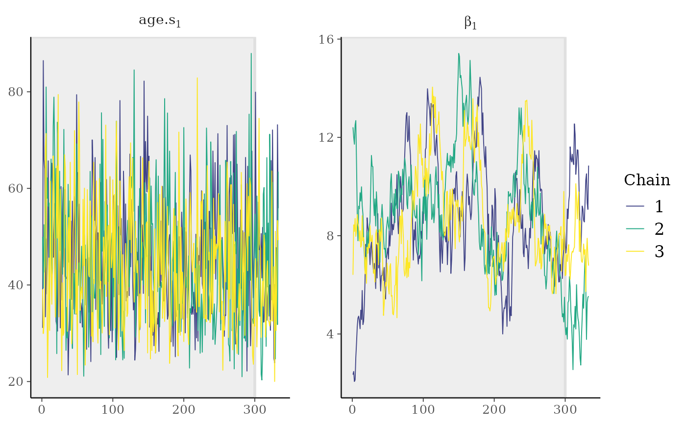

The left panel gives an impression how well-mixed chains should look like for the first of the estimated ages. On contrast, the right panel illustrates chains for the parameter beta, the slope of the latent linear regression function, that have not yet well-mixed. Longer chains are clearly necessary. This can also be illustrated with a plot showing the Potential scale reduction factor (PSRF), already mentioned above:

coda::gelman.plot(sorsum_as_res[, c("b", "beta[1]")])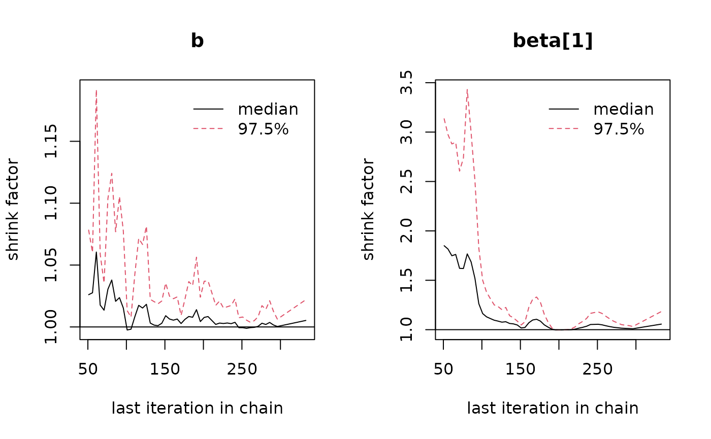

Ideally, the value of the PSRF should converge to 1, but stay below 1.1. On the left panel for the parameter b, this is clearly the case, but not so on the right panel, again for the beta parameter (please note the difference in scale of the y-axis!). This therefore also indicates that more iterations are required.

From the minimum ESS value of around 25 (see above), it can be surmised that roughly 400 times more iterations are needed to get to a value of 10,000. This would increase runtime proportionally (approximately 200–250 minutes, equaling about 4 hours). However, because the resulting file would also be 400 times larger, some degree of thinning is necessary, so saving only, say, every 10,000th step (= thinning of 10,000). This in turn might increase autocorrelation which in turn will force you to run the model even longer.

In the current vignette, we forego this step at the moment. Instead, we inspect the seven thresholds between the eight levels. For this, we use the internal function threshold.chains() to compute the threshold values for each iteration. The computation of the thresholds on the age-scale is done outside of the MCMC simulation to reduce computational cost and memory usage. The function returns a coda::mcmc.list() which is further processed with first diagnostic.summary() and then threshold.matrix(). The latter is again a convenience function to extract mean thresholds values from the output of diagnostic.summary() which is particularly handy when dealing with several traits.

thresholds <- threshold.chains(sorsum_as_res)
thresh_diag <- diagnostic.summary(thresholds)
threshold.matrix(thresh_diag) |> data.frame() |> knitr::kable(digits = 1)

X1	X2	X3	X4	X5	X6	X7
18	21.5	29.3	49.4	70.4	76.8	83.8

The thresholds of this trait (auricular surface) are unevenly spaced within the age range of 18 and 100 years. The probability distribution of the thresholds can conveniently visualised with e.g. the R-package bayesplot. To avoid too glaring colors, we switch the color scheme again:

bayesplot::color_scheme_set("gray")
bayesplot::mcmc_areas_ridges(thresholds, prob = 0.8, point_est = c("median"), 
                      border_size = 0.2) + 
  theme_light() + xlim(18,100) + labs(x = "\nage-at-death (years)")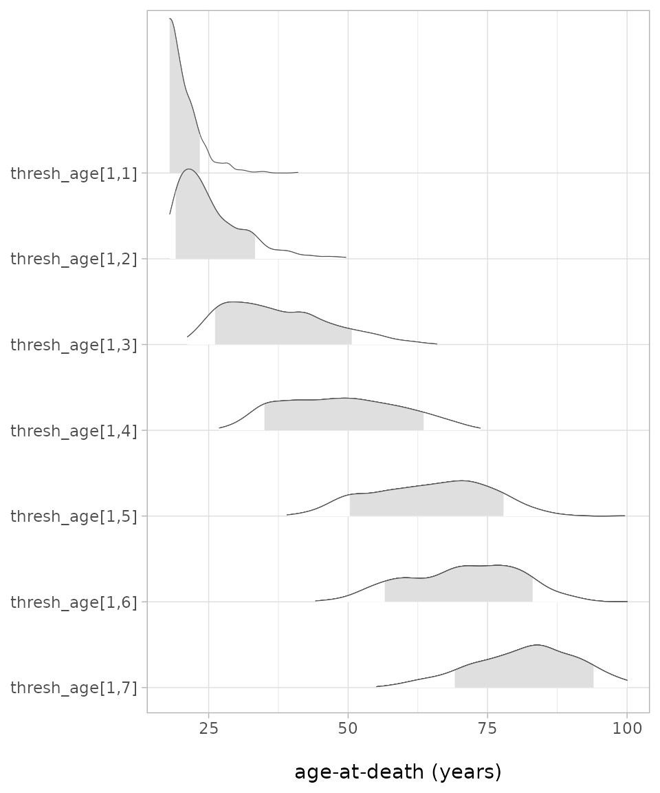

The resulting plot shows impressively the considerable overlap between the thresholds, even when only the 80%-credible level is shown (grey shaded areas), but also again that the thresholds are not evenly spaced. Interesting would be a comparison with the thresholds of this trait computed for other populations, keeping in mind that the current values are not reliable as the quality measures were not yet met.

The function age.estim.summary() conveniently provides summaries of age-related quantities like the mean estimated age, the mean of the highest density interval of the estimated ages as well as the parameters $\alpha$ , $\beta$ , and - derived from these two – the modal age M:

age.estim.summary(sorsum_as_res_diag) |> knitr::kable(digits = 3)

	Mean	Median	Mode	0.025	0.975
b	0.044	0.041	0.029	0.020	0.075
a	0.009	0.007	0.003	0.000	0.023
M	55.407	60.176	70.585	17.155	81.774
age_mean	56.467	57.851	58.185	23.859	82.933
hdi_diff	41.918	45.582	46.995	17.680	50.300

The above table demonstrates that it makes a difference whether you choose Mean, Median or Mode as the measure of the mean.

To illustrate the distribution of some of the individual ages, this time we rely on the functionality of the R package tidybayes (Kay 2024). Its function tidybayes::spread_draws() allows to subset the chains in a single step to extract the estimated ages (age.s). We limit here the age estimates to the first seven.

sorsum_as_res |> tidybayes::spread_draws(age.s[age_number])  |> 
  subset(age_number < 8) |>
  ggplot(aes(y =  as.factor(age_number), x = age.s)) +
  tidybayes::stat_halfeye(
    .width = 0.95, point_interval = mode_hdi, fill = "lightgrey") + 
  scale_x_continuous(breaks = seq(10,100,10), limits = c(18, 100)) +
  labs( x = "\nModal age-at-death (years)", y = "Individual no.\n" ) + 
  theme_light() +
  theme(panel.grid.minor.x = element_blank(), text = element_text(size = 12))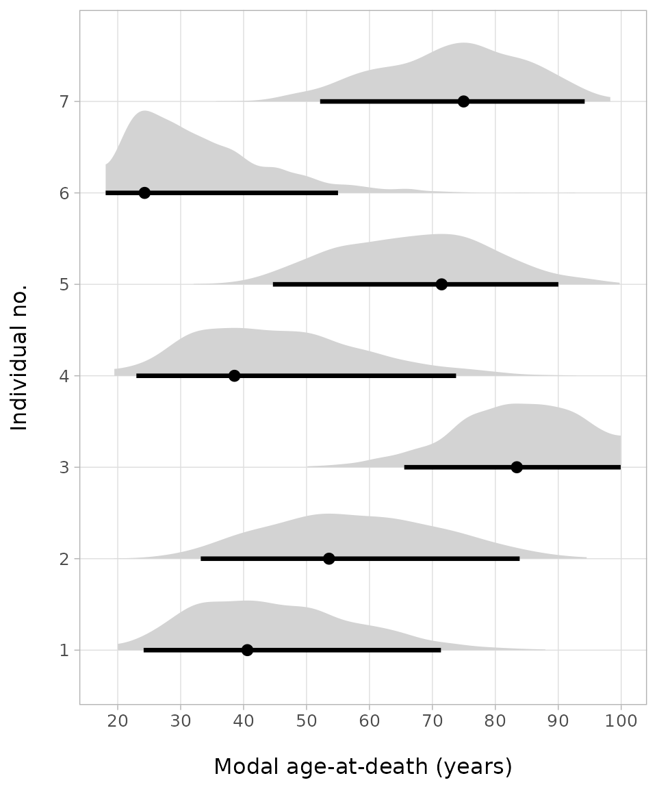

The plots of the first seven age estimates look similar to the threshold plots and allow immediate assessment of the spread of the probability distribution of the age estimates. So, for example, for the first individual with stage 4 of the auricular surface, the age mode is at about 40 years, but the 95%-credible range is between about 25 to 70 years.

Together with the individual age-at-death estimates, bay.ta() also estimates the parameters of the underlying Gompertz function, $\alpha$ and $\beta$ :

ggplot() + ylab("density\n") + 
  geom_function(fun =  function(x) 
    flexsurv::dgompertz(x - 18, sorsum_as_res_diag["b",3],
                        sorsum_as_res_diag["a",3])) +
  xlab("\nAge in years") + theme_light() +
  scale_x_continuous(breaks = seq(10,100,10), limits = c(18, 100)) +
  theme(panel.grid.minor.x = element_blank(), text = element_text(size = 12))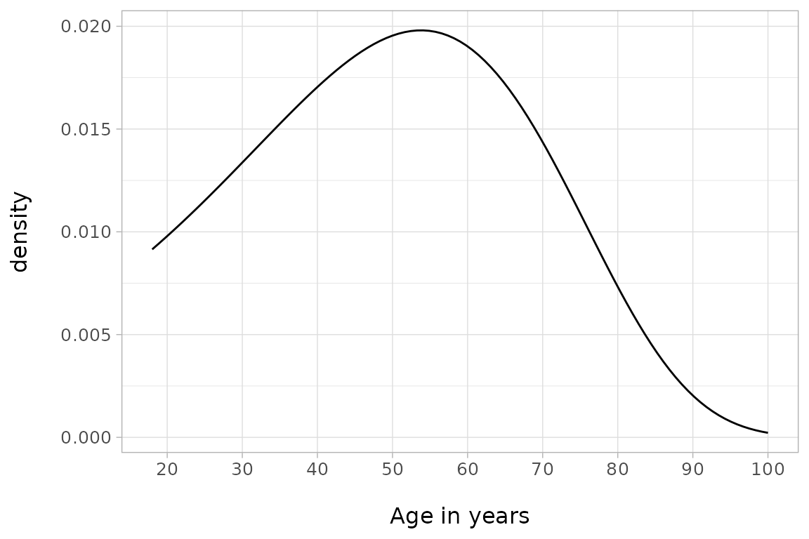

The Gompertz function provides a different perspective on the mortality structure of the population studied as it does not depend on individual point estimates of ages like, for example, Kaplan-Meier-diagrams. Please note that the maximum of the curve coincides with the arithmetic mean of the modal age M (55 years) in the table above.

Running the analysis with JAGS

Provided JAGS is installed, bay.ta() can also be run with JAGS. For this, it is sufficient to set the parameter framework to JAGS. All other parameters remain unchanged.

sorsum_as_res <- bay.ta(
  framework = "JAGS",
  method = sorsum_as[,2],
  minimum_age = 18,
  thinSteps = 100,
  numSavedSteps = 5000,
  seed = 1234
)

The JAGS model needs a little bit longer than the NIMBLE model but if you run the diagnostics you will see that the overall performance is superior. At this point, we leave the further analysis following the same steps as above to the reader.

Going further

More vignettes explain framework decisions (vignette("computation_framework")), detail the model in mathematical terms (vignette("mathematical_background")), demonstrate how data sets with known age-at-death can be dealt with (vignette("known_age")), provide a thoroughly worked example (vignette("articles/worked_example")) and show how the posterior probability densities can be grouped (vignette("articles/groupings")).

References

Gabry, Jonah, Daniel Simpson, Aki Vehtari, Michael Betancourt, and Andrew Gelman. 2019. “Visualization in Bayesian Workflow.” Journal of the Royal Statistical Society A 182: 389–402. https://doi.org/10.1111/rssa.12378.

Kay, Matthew. 2024. tidybayes: Tidy Data and Geoms for Bayesian Models. https://doi.org/10.5281/zenodo.1308151.

Kruschke, John K. 2015. Doing Bayesian data analysis: a tutorial with R, JAGS, and Stan. Academic Press.

Lovejoy, C. Owen, Richard S. Meindl, Thomas R. Pryzbeck, and Robert P. Mensforth. 1985. “Chronological metamorphosis of the auricular surface of the ilium: A new method for the determination of adult skeletal age at death.” American Journal of Physical Anthropology 68 (1): 15–28. https://doi.org/10.1002/ajpa.1330680103.

Moser, Daria, Sandra L. Pichler, Ana Luisa Santos, Florian Klimscha, and Katharina Fuchs. 2025. “The uncertain death. Estimating mortality structure by random sampling.” International Journal of Osteoarchaeology 35 (1): e3363. https://doi.org/10.1002/oa.3363.

Müller-Scheeßel, Nils, Christoph Rinne, and Katharina Fuchs. 2026. “A Fully Bayesian Approach to Adult Skeletal Age Estimation: Multivariate Latent Trait Modeling with Markov Chain Monte Carlo Sampling.” American Journal of Biological Anthropology.