Introduction
While bay.ta() estimates age at the individual level,
many research questions operate at the group level (e.g., comparing
burial populations or social categories). Because bay.ta()
does not (yet) contain a grouping variable as would be the case in a
hierarchic model, the following approach aggregates posterior age
distributions post hoc without modifying the underlying model.
In this way, we can compare sub-groups within one data set. This purpose
serves the helper function prob.cat(). We demonstrate its
functioning here with the two variables AGE and
SEX of the osteological analysis of Chelsea ‘Old church’.
More meaningful choices could be sub-populations according to location,
burial customs or grave goods. However, the principle would be the
same.
Downloading the data
We re-use here the data already used for the vignette on Chelsea ‘Old
church’ (vignette("worked_example")). So, the respective
MCMC data is downloaded from a Github repository.
path <- "https://raw.githubusercontent.com/ISAAKiel/Chelsea_mcmc/main/"
file <- "chelsea_complete_cal_res.Rdata"
temp <- tempfile()
if (Sys.info()[["sysname"]] == "Darwin") {
  download.file(paste0(path, file), destfile = temp, method = "curl", mode = "wb")
} else {
  download.file(paste0(path, file), destfile = temp, method = "libcurl", mode = "wb")
}
con <- gzfile(temp, "rb")
load(con)
close(con)
Probability densities in practice
Data input to prob.cat()
Apart from the coda::mcmc.list() resulting from
bay.ta(), prob.cat() expects a character
string (age_identifier) specifying the row name of the age
estimates (either age.s or age.s_c as here), a
vector of the grouping variable (group_vec) which needs to
be of the same length as the number of age estimates and a specification
of the mode switch. The summed option produces a pooled
(mixture) distribution of all individuals within a group, reflecting the
combined posterior probability mass. In contrast, mean
averages the posterior values across individuals per iteration, yielding
a distribution of group-level central tendencies. The results are
visualized with ggplot2 (Wickham
2016) and the additional packages tidybayes (Kay 2024), ggpubr (Kassambara 2025), and ggridges
(Wilke 2025).
For the blue vertical lines in the left plots below, we need a column for the estimated ages. Again, we recycle here code from the vignette on Chelsea that adds this column to the original data.
chelsea_complete_cal_diag <-
    diagnostic.summary(chelsea_complete_cal_res)
chelsea_complete_cal_diag_red_ages <-
  chelsea_complete_cal_diag[grep("^age.s_c",
                                 rownames(chelsea_complete_cal_diag)),]
chelsea_complete$estimated_age <-
  round(chelsea_complete_cal_diag_red_ages[,5],1)
Chelsea ‘Old church’: Age
As first example, we group the posterior probability densities by the osteological age categories as determined by the team of the Museum of London. Since both approaches rely on the same underlying traits, a broad agreement is expected, although systematic differences may arise from the probabilistic modelling and calibration.
chelsea_summed_prob_age <- prob.cat(mcmc_list = chelsea_complete_cal_res,
                                  age_identifier = "age.s_c",
                                  group_vec = chelsea_complete$AGE,
                                  mode = "summed")
chelsea_mean_prob_age <- prob.cat(mcmc_list = chelsea_complete_cal_res,
                                    age_identifier = "age.s_c",
                                  group_vec = chelsea_complete$AGE,
                                    mode = "mean")
ggpubr::ggarrange(
  ggplot(chelsea_summed_prob_age, aes(x = x, y = category, height = y)) +
    ggridges::geom_density_ridges(
      stat = "identity",
      colour = "darkgrey",
      fill = "lightgrey",
      alpha = 0.7,
      scale = 0.9,
      rel_min_height = 0.01
    ) +
    scale_x_continuous(limits = c(18, 100), breaks = seq(20, 100, by = 10)) +
    xlab("Probability density of estimated age") +
    ylab("Age category") +
    scale_y_discrete(expand = expansion(mult = c(0.05, 0.3))) +
    ggridges::theme_ridges(font_size = 11) +
    geom_point(
      data = chelsea_complete,
      aes(x = estimated_age, y = as.numeric(AGE) + 0.075),
      color = "blue", shape = '|', size = 4, alpha = 0.8,
      position = position_jitter(height = 0), inherit.aes = FALSE
    ),
  ggplot(chelsea_mean_prob_age, aes(x = value, y = category)) +
    tidybayes::stat_halfeye(
      .width = 0.95,
      adjust = 0.6,
      slab_size = 0.6,
      point_interval = tidybayes::mode_hdi,
      slab_colour = "darkgrey",
      fill = "lightgrey",
      linewidth = 0.8
    ) +
    scale_x_continuous(limits = c(18, 100), breaks = seq(20, 100, by = 10)) +
    xlab("Posterior mean age") +
    ylab("Age category") +
    scale_y_discrete(expand = expansion(mult = c(0.05, 0.3))) +
    ggridges::theme_ridges(font_size = 11)
)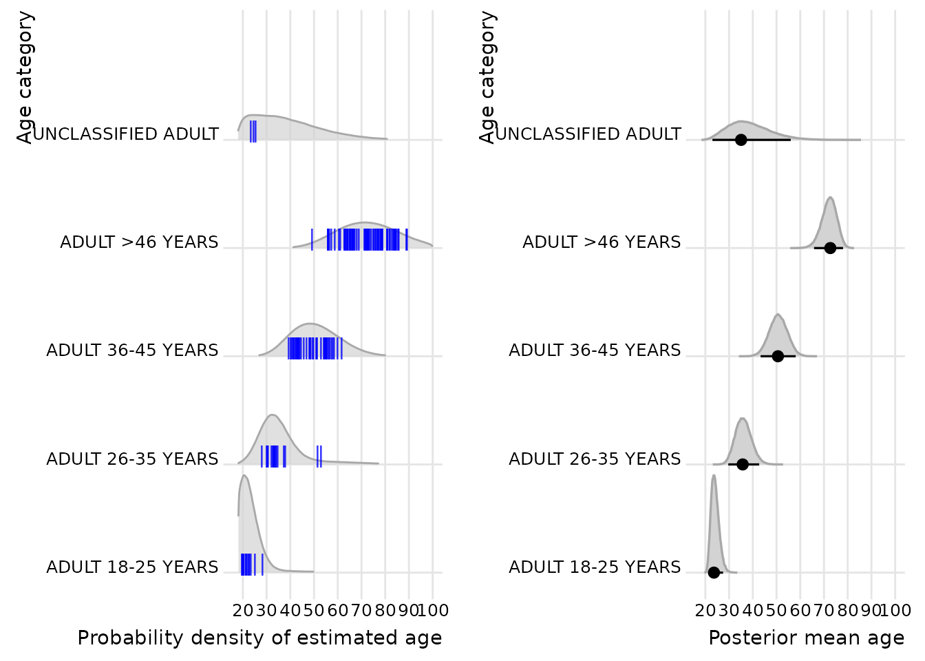
The left plot displays summed probability densities of all estimates of one osteological age group combined with the mode of the individual estimates as blue short vertical lines. The densities are normalized within each group and therefore do not reflect group size. The plot somehow resembles similar plots of calibrated C14 data. The overall agreement between the osteological age estimates and the Bayesian estimates is very good. However, a close inspection shows that especially the age group 36–45 years according to the Bayesian estimates extends far beyond the proposed limit of 45 years. This suggests that the traditional age category may truncate older individuals whose trait expressions overlap with higher age ranges. In the right plot the mean of this age group is fixed at about 50 years. The means of the other age groups are within the limits of the osteological age ranges, though at the upper range.
Chelsea ‘Old church’: Sex
The second example groups the probability densities according to the sex determinations.
chelsea_summed_prob_sex <- prob.cat(mcmc_list = chelsea_complete_cal_res,
                                  age_identifier = "age.s_c",
                                  group_vec = chelsea_complete$SEX,
                                  mode = "summed")
chelsea_mean_prob_sex <- prob.cat(mcmc_list = chelsea_complete_cal_res,
                                    age_identifier = "age.s_c",
                                    group_vec = chelsea_complete$SEX,
                                    mode = "mean")

ggpubr::ggarrange(
  ggplot(chelsea_summed_prob_sex, aes(x = x, y = category, height = y)) +
    ggridges::geom_density_ridges(
      stat = "identity",
      colour = "darkgrey",
      fill = "lightgrey",
      alpha = 0.7,
      scale = 0.9,
      rel_min_height = 0.01
    ) +
    scale_x_continuous(limits = c(18, 100), breaks = seq(20, 100, by = 10)) +
    xlab("Probability density of estimated age") +
    ylab("Sex category") +
    scale_y_discrete(expand = expansion(mult = c(0.05, 0.3))) +
    ggridges::theme_ridges(font_size = 11) +
    geom_point(
      data = chelsea_complete,
      aes(x = estimated_age, y = as.numeric(SEX) + 0.075),
      color = "blue", shape = '|', size = 4, alpha = 0.8,
      position = position_jitter(height = 0), inherit.aes = FALSE
    ),

  ggplot(chelsea_mean_prob_sex, aes(x = value, y = category)) +
    tidybayes::stat_halfeye(
      .width = 0.95,
      adjust = 0.6,
      slab_size = 0.6,
      point_interval = tidybayes::mode_hdi,
      slab_colour = "darkgrey",
      fill = "lightgrey",
      linewidth = 0.8
    ) +
    scale_x_continuous(limits = c(18, 100), breaks = seq(20, 100, by = 10)) +
    xlab("Posterior mean age") +
    ylab("Sex category") +
    scale_y_discrete(expand = expansion(mult = c(0.05, 0.3))) +
    ggridges::theme_ridges(font_size = 11)
)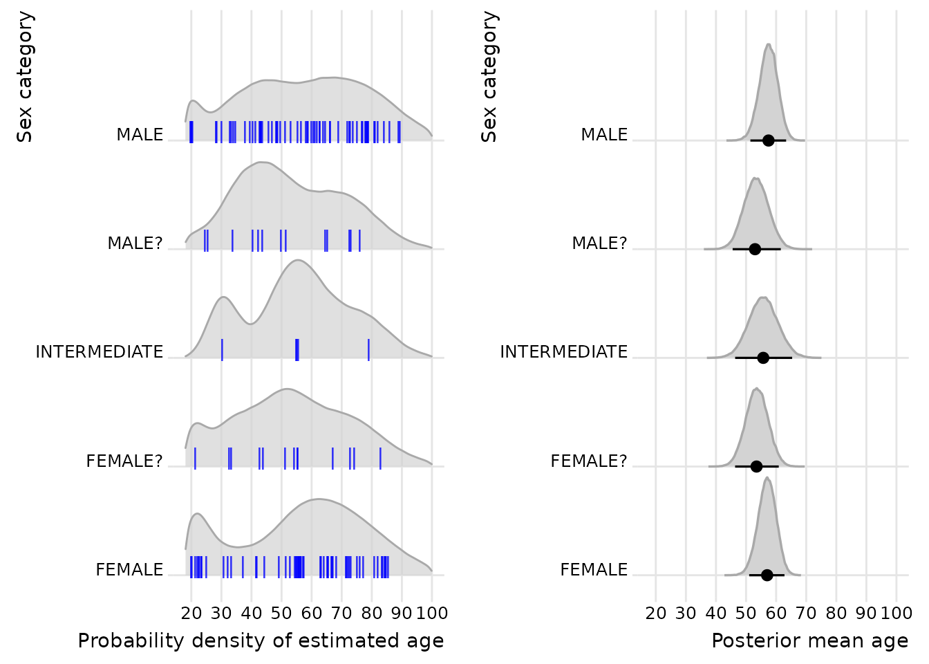
Compared to AGE, the SEX groups display no
clear pattern. Their means on the right plot are all around 55 years,
and their highest density intervals, the black line at the
bottom of the densities extending to the left and right from the black
circle, overlap to a large extent. The lack of systematic differences
between sex categories suggests that the estimated age distributions are
largely independent of osteological sex classification in this data set.
Nevertheless, the bimodal distribution of the females raises some
questions. It seems possible that the peak in their 20s reflects
heightened maternal mortality or that access to the crypt favored either
very young or comparatively old women.
Overall, the examples above illustrate how posterior age distributions can be flexibly aggregated to explore group-level patterns and assess how posterior age distributions vary across categorical variables without modifying the underlying model.