Chelsea 'Old Church': A worked example

Load libraries

library(baytaAAR)
library(dplyr)
library(tidyr)
library(ggplot2)

The churchyard of All Saints, Chelsea’s Old Church

Introduction

For the worked example to show the complete range of functions provided by baytaAAR, we chose the churchyard of All Saints, Chelsea’s Old Church (Cowie et al. 2008). For an overview of the site and the osteological investigations, see the respective website of the Museum of London.

The data of the osteological team of the Museum of London is freely available, including the age estimations and especially the raw scores that formed the basis for the finally published age ranges. If possible, the team applies four established age estimation methods to the human remains: Dental wear with Codes 1-4, Pubic symphysis with Phases I-VI, Auricular surface with Phases 1-8, and Costochondral with Phases 0-8. For the background of these methods and their application, see again the respective website of the Museum of London. From the complete Chelsea dataset, we chose those individuals where at least one of the four methods was applicable. As a special feature of this churchyard, for some of these individuals the age-at-death is known thanks to plates on the coffins.

This worked example proceeds in five steps: (1) data preparation, (2) single-trait models, (3) multivariate models, (4) model comparison and calibration, and (5) evaluation against known ages. One of the main aims is to sketch the process to arrive at plausible age estimates in terms of highest density intervals when the data set contains a lot of missing instances. The complete-case model best captures joint trait covariance without imputation, hence provides the least biased estimate of the underlying uncertainty structure.

Loading data

The first step is the loading and preparation of the data. For that, we download and extract the data directly from the website of the Museum of London and extract it. The second table contains known age-at-death for some of the individuals from plates on the coffins. We then filter only the adults and expand the age estimation table. The two tables are merged and only the CONTEXT column with the individual number, the sex and age estimation as well as the raw age estimations code and the known age-at-death column are retained. Finally, all entries 9, which for all four age estimations methods equal undecided, are converted to NA and only those rows with at least one valid method are kept.

temp <- tempfile()
download.file(
  "https://dams.londonmuseum.org.uk/m/2dc89b01e62759ff/original/PMCOC.zip",
  temp, mode = "wb")
unzip(temp, "PMCOC_age_estimates.lst")
chelsea_age <- read.delim("PMCOC_age_estimates.lst",
                          sep = "|",
                          header = TRUE,
                          stringsAsFactors = FALSE,
                          row.names = NULL,
                          fill = TRUE,
                          strip.white = TRUE)

# absolute ages according to Cowie et al. 2008, 41 table 6
chelsea_known_age <- data.frame(
  CONTEXT = c(35, 147, 198, 462, 525, 622, 654, 681, 701, 713,
              722, 744, 792, 976, 980, 990, 1133),
  known_age = c(60, 67, 44, 61, 70, 84, 66, 84, 78, 68, 56, 70,
                68, 82, 54, 32, 70) )

chelsea_age_col <- colnames(chelsea_age)[-7]
chelsea_age <- chelsea_age[,-14]
colnames(chelsea_age) <- chelsea_age_col

chelsea_adults <- 
  chelsea_age |> dplyr::filter(grepl("^(ADULT|UNCLASSIFIED ADULT)", AGE))

chelsea_adults_wide <- chelsea_adults |>
  dplyr::mutate(VALUE = as.numeric(VALUE)) |>
  tidyr::pivot_wider(
    id_cols = c(CEMETERY, SITECODE, PERIOD, LU_INT, E_DATE, L_DATE,
                CONTEXT, SEX, AGE, TRAIT_TYPE),
    names_from = EXPANSION,
    values_from = VALUE
  )

# combine both tables
chelsea <- merge(chelsea_adults_wide, chelsea_known_age,
                     by = "CONTEXT",
                     all.x = TRUE)

# limit data set to relevant columns
chelsea_mat <- chelsea[,c(1, 8, 9, 12,13,14,15,18)]

chelsea_mat[chelsea_mat == 9] <- NA
chelsea_complete <- chelsea_mat[rowSums(is.na(chelsea_mat[,4:7])) != 4, ]
chelsea_complete$AGE <- factor(chelsea_complete$AGE,
                               levels = c("ADULT 18-25 YEARS",
                                          "ADULT 26-35 YEARS",
                                          "ADULT 36-45 YEARS",
                                          "ADULT >46 YEARS",
                                          "UNCLASSIFIED ADULT"),
                               ordered = TRUE)
chelsea_complete$SEX <- factor(chelsea_complete$SEX,
                          levels = c("FEMALE",
                                     "FEMALE?",
                                     "INTERMEDIATE",
                                     "MALE?",
                                     "MALE"),
                          ordered = TRUE)

# define data sets with specific traits
chelsea_no_nas <- chelsea_complete[rowSums(is.na(
  chelsea_complete[,4:7])) == 0, ]
chelsea_ps_as <- 
  chelsea_complete[rowSums(is.na(chelsea_complete[,5:6])) == 0, ]
chelsea_dental <- chelsea_complete[(!is.na(chelsea_complete[,4])), ]
chelsea_ps <- chelsea_complete[(!is.na(chelsea_complete[,5])), ]
chelsea_as <- chelsea_complete[(!is.na(chelsea_complete[,6])), ]
chelsea_costo <- chelsea_complete[(!is.na(chelsea_complete[,7])), ]

# show first lines, replace underscore with space for variable "known_age"
head(chelsea_complete) |> 
  knitr::kable (col.names = gsub("[_]", " ", names(chelsea_complete)))

CONTEXT	SEX	AGE	Dental wear (Codes 1-4)	Pubic symphysis Phases I-VI	Auricular surface Phases 1-8	Costochondral Phases 0-8	known age
18	FEMALE	ADULT 36-45 YEARS	1	4	4	5	NA
19	FEMALE	ADULT >46 YEARS	3	5	8	NA	NA
20	MALE	ADULT 36-45 YEARS	3	5	4	NA	NA
31	FEMALE	ADULT 36-45 YEARS	NA	5	6	5	NA
35	MALE	ADULT >46 YEARS	1	5	6	6	60
39	FEMALE	ADULT 36-45 YEARS	NA	5	5	5	NA

The table above gives an impression of the data structure of the Chelsea individuals with estimated sex and age, the four traits used for estimations as well as a last column with known age-at-death for a few individuals.

Descriptive statistics

Next, we want to get an overview of the number of individuals, the sex estimations and especially the number of phases for each method.

chelsea_complete |> nrow()
#> [1] 152

All in all, there are at least 152 individuals with information on at least one method.

chelsea_complete[,2] |> table()
#> 
#>       FEMALE      FEMALE? INTERMEDIATE        MALE?         MALE 
#>           57           13            5           13           64

Based on the osteological sex estimations, it seems that both sexes are present in roughly equal numbers. The known-age structure is as follows:

chelsea_complete$known_age |> na.omit() |> as.numeric() |> sort()
#>  [1] 32 44 54 56 60 61 66 67 68 68 70 70 70 78 84 84

Most of the 16 individuals with known age-at-death are at least 60 years or above. There are only four individuals with a plate of younger age.

The following code produces an overview of the age estimations methods and the counts per phase of each method, including the number of NAs:

options(knitr.kable.NA = '')
chelsea_complete |>
  dplyr::select(starts_with("Dental"),
         starts_with("Pubic"),
         starts_with("Auricular"),
         starts_with("Costo")) |>
  tidyr::pivot_longer(everything(), names_to = "method", values_to = "phase") |>
  dplyr::mutate(phase = as.character(phase)) |>
  dplyr::count(method, phase) |>
  tidyr::pivot_wider(names_from = phase, values_from = n, values_fill = NA) |>
  knitr::kable ()

method	1	2	3	4	5	6	7	8	NA
Auricular surface Phases 1-8	6	8	12	23	28	20	16	18	21
Costochondral Phases 0-8	3	4	3	3	11	7	17	6	98
Dental wear (Codes 1-4)	27	15	6	16					88
Pubic symphysis Phases I-VI	11	4	4	13	35	27			58

The overview shows that the costochondral is the method with the least applicability (= most NAs) while the method with the least NAs is the auricular surface, followed by the pubic symphysis. Dental wear was possible to determine only in a few cases more than the costochondral. All in all, the missing information is considerable:

count_na <- sum(is.na(chelsea_complete[,4:7]))
count_cells <- nrow(chelsea_complete) * 4
round(count_na / count_cells * 100,1)
#> [1] 43.6

Overall, more than 40 percent of the cells are NA. This level of missingness is expected to affect multivariate models via imputation uncertainty.

Running `baytaAAR`

We will now analyse the Chelsea data with baytaAAR systematically. This implies to analyse all methods separately and then together. We will do the following runs, also indicate if we use the JAGS or NIMBLE version as well as either norm (multiple normal) or mnorm (multinormal) in case of the inclusion of more than one method in the same run. The difficulty here is that many entries, as shown above, are NA. These will be a challenge for the multinormal analysis as the unobserved nodes will have to be imputed. We will compare a minimum set of individuals where all four methods are present with a maximum set of the two most common methods, auricular surface and pubic symphysis.

only auricular surface (with JAGS)
only costochondral (with JAGS)
only dental wear (with JAGS)
only pubic symphysis (with JAGS)
all methods and only individuals with all methods present (with NIMBLE and mnorm)
only auricular surface and pubic symphysis and only individuals with both methods present (with NIMBLE and mnorm)
all methods and all individuals (with NIMBLE and mnorm)
all methods and all individuals with calibration term (with JAGS)

Defining paths for downloading RDA-files

Please note that the models should run until the resulting Markov Chain Monte Carlo (MCMC) samples meet certain quality criteria. As already noted in the introductory article (vignette("baytaAAR")), these are 10,000 for ESS and below 1.1 for PSRF. To spare the time in running the models, we saved RDA-files with the raw MCMC-chains on Github for downloading and loading. If you really want to run the models, set runNewMCMC to TRUE. If not, stick to the negation !TRUE.

runNewMCMC = !TRUE
path <- "https://raw.githubusercontent.com/ISAAKiel/Chelsea_mcmc/main/"

Only single traits (with `JAGS`)

We first concentrate on only those individuals where the auricular surface was assessable. The first argument method is the trait which are used for age estimation, the auricular surface in this case. The data has to be of the class matrix. minimum_age and maximum_age truncate the underlying Gompertz distribution to a reasonable range. parameters denotes the estimated and monitored variables. They have the following meaning:

b: Gompertz beta
a: Gompertz $\alpha$ , in bay.ta linked deterministically to Gompertz $\beta$ to reduce volatility
beta0: the intercept of the latent continuous variable underlying the ordinal trait
beta: the slope of the latent continuous variable underlying the ordinal trait
thresh: the threshold value. The number of thresholds equals the number of levels of the trait minus 1
age.s: the estimated age of each individual

The rest of the variables control JAGS. multicore specifies here that the code is executed in parallel for speed. thinSteps controls the amount of thinning of the resulting Markov Chain. With 1 there is no thinning. However, because the ordered probit model suffers from high auto-correlation, this number will almost certainly not suffice. Setting the number of numSavedSteps too high might lead to overly large files. Therefore, it is always a good idea to start with a moderate value for numSavedSteps of about 10,000 and a value for thinSteps of 1, and then increase the number of steps according to the first result. A future version of baytaAAR might also include the possibility to define quality goals which the code should reach. Finally, we run bay.ta with a seed for reproducibility

if ( runNewMCMC ) {
  chelsea_as_res <- bay.ta(
    framework = "JAGS",
    method = chelsea_as[,6],
    minimum_age = 18,
    maximum_age = 100,
    parameters = c( "b", "a", "beta0", "beta", "thresh", "age.s"),
    multicore = TRUE,
    thinSteps = 10000, # necessary 10000, takes 16 hours
    numSavedSteps = 80000,
    seed = 3901)
} else {
  file <- "chelsea_as_res.Rdata"
  temp <- tempfile()
  download.file(paste0(path, file), destfile = temp, mode = "wb")
  con <- gzfile(temp, "rb")
  load(con)
  close(con)
  threshold_as <- chelsea_as_res |> threshold.chains() |> 
  diagnostic.summary() |> threshold.matrix(mean_choice = "Mode")
}

The resulting Markov chains are stored in the file chelsea_as_res in the coda::mcmc.list() format for further processing. The function diagnostic.summary() provides a summary of the posterior estimates:

chelsea_as_diag <- diagnostic.summary(chelsea_as_res)
head(chelsea_as_diag[-c(9:12),], 20) |>  knitr::kable (digits = 4)

	PSRF Point est.	PSRF Upper C.I.	Mean	Median	Mode	ESS	MCSE	HDImass	HDIlow	HDIhigh
M	1.0000	1.0002	45.4775	47.4925	59.4297	70546.7	0.0773	0.95	6.1069	78.5853
b	1.0002	1.0006	0.0363	0.0323	0.0233	52284.1	0.0001	0.95	0.0200	0.0662
a	1.0000	1.0002	0.0128	0.0125	0.0075	70383.0	0.0000	0.95	0.0002	0.0254
beta0	1.0003	1.0008	-21.5060	-21.3985	-20.6710	15523.4	0.0535	0.95	-34.7759	-8.5747
beta	1.0003	1.0007	7.1481	7.1100	6.9539	14376.5	0.0178	0.95	3.0347	11.4485
thresh[1,1]			0.5000	0.5000	0.4997	0.0		0.95	0.5000	0.5000
thresh[1,2]	1.0002	1.0006	1.9635	1.8432	1.6870	31420.5	0.0037	0.95	0.9120	3.2764
thresh[1,3]	1.0001	1.0003	3.4145	3.2799	3.0093	20018.1	0.0073	0.95	1.5951	5.4751
age.s[1]	1.0000	1.0001	41.1489	38.4174	33.3702	58974.5	0.0514	0.95	22.2436	68.0039
age.s[2]	1.0000	1.0000	78.8939	79.4970	80.5174	78982.0	0.0387	0.95	60.1759	99.9917
age.s[3]	1.0000	1.0001	41.1413	38.3824	33.2010	55738.3	0.0531	0.95	21.5114	67.7183
age.s[4]	1.0001	1.0002	60.6264	59.5504	57.3965	74371.7	0.0451	0.95	38.8846	85.6228
age.s[5]	1.0001	1.0003	60.5946	59.5239	56.9639	76916.6	0.0443	0.95	38.2957	85.2045
age.s[6]	1.0000	1.0001	51.3528	49.4329	44.5627	65909.4	0.0504	0.95	29.8255	78.6532
age.s[7]	1.0000	1.0002	68.3786	68.0310	66.6683	78557.4	0.0411	0.95	46.7133	90.9865
age.s[8]	1.0001	1.0001	22.4139	20.6652	18.6010	39476.1	0.0302	0.95	18.0001	32.2237
age.s[9]	1.0005	1.0008	27.2808	24.6971	21.9435	40673.9	0.0442	0.95	18.0006	45.0100
age.s[10]	1.0001	1.0003	51.3471	49.3553	44.5884	65944.7	0.0504	0.95	29.1614	77.8690
age.s[11]	1.0001	1.0004	51.3272	49.4402	44.3857	64014.4	0.0509	0.95	29.3780	77.9389
age.s[12]	1.0000	1.0002	51.3263	49.3472	45.0358	67410.5	0.0496	0.95	29.9367	78.3928

The above table just shows a part of the full diagnostic table. Especially when many parameters are to be estimated, it can contain quite a number of rows. The columns show a summary of the individual estimates of each parameter with the following meaning:

PSRF Point est.: Potential scale reduction factor (= Gelman-Rubin statistic), a measure of the mixing of chains.
PSRF Upper C.I.: The upper limit of the 0.95-confidence interval of the PSRF.
Mean: Arithmetic mean of the estimates.
Median: Median of the estimates.
Mode: Mode of the estimates.
ESS: Effective sample size, a control of autocorrelation.
MCSE: Monte Carlo standard error.
HDImass: Credibility level of the highest density interval
HDIlow: Start of the highest density interval.
HDIhigh: End of the highest density interval.

For more information on these measures, the reader is referred to e.g. the book “Doing Bayesian data analysis” by J. Kruschke (2015). The summary tool diagnostics.max.min quickly allows to see the worst values:

chelsea_as_diag |> diagnostics.max.min()
#>   PSRF_max PSRF_upper_max ESS_min
#> 1 1.001342       1.001833 13766.8

The highest PSRF value is clearly far below 1.1 and the lowest ESS value higher than 10,000. We are therefore safe to proceed with the analysis and to calculate a summary of the age estimates:

chelsea_as_age_ranges <- age.estim.summary(chelsea_as_diag)
chelsea_as_age_ranges |>  knitr::kable(digits = 3)

	Mean	Median	Mode	0.025	0.975
b	0.036	0.032	0.023	0.020	0.066
a	0.013	0.012	0.007	0.000	0.025
M	45.478	47.492	59.430	6.107	78.585
age_mean	52.354	51.339	51.805	22.416	78.893
hdi_diff	42.279	46.080	46.965	14.249	48.762

From the diagnostics, the baytaAAR helper function age.estim.summary() computes, for example, that the average mean, median and mode of the age range estimated from the data is hovering around 45 years. This might seem like a very large range (and it certainly is!) but the model promises that this credible range contains 95% of the true ages-at-death.

We will now proceed with the other traits and look again at the auricular surface when comparing its results with the other runs. The models for the other single traits are not discussed in detail as they only mirror the approach for the auricular surface. We will examine their results when all model runs have been completed.

if ( runNewMCMC ) {
  chelsea_ps_res <- bay.ta(
    framework = "JAGS",
    method = chelsea_ps[,5],
    minimum_age = 18,
    maximum_age = 100,
    parameters = c( "b", "a", "beta0", "beta", "thresh", "age.s"),
    multicore = TRUE,
    thinSteps = 2000,
    numSavedSteps = 100000,
    seed = 991)
} else {
  file <- "chelsea_ps_res.Rdata"
  temp <- tempfile()
  download.file(paste0(path, file), destfile = temp, mode = "wb")
  con <- gzfile(temp, "rb")
  load(con)
  close(con)
}
chelsea_ps_diag <- diagnostic.summary(chelsea_ps_res)
chelsea_ps_age_ranges <- age.estim.summary(chelsea_ps_diag)
threshold_ps <- chelsea_ps_res |> threshold.chains() |> 
  diagnostic.summary() |> threshold.matrix(mean_choice = "Mode")

if ( runNewMCMC ) {
  chelsea_costo_res <- bay.ta(
    framework = "JAGS",
    method = chelsea_costo[,7],
    minimum_age = 18,
    maximum_age = 100,
    parameters = c( "b", "a", "beta0", "beta","thresh","age.s"),
    multicore = TRUE,
    thinSteps = 1500,
    numSavedSteps = 100000,
    seed = 6433)
} else {
  file <- "chelsea_costo_res.Rdata"
  temp <- tempfile()
  download.file(paste0(path, file), destfile = temp, mode = "wb")
  con <- gzfile(temp, "rb")
  load(con)
  close(con)
}
chelsea_costo_diag <- diagnostic.summary(chelsea_costo_res)
chelsea_costo_age_ranges <- age.estim.summary(chelsea_costo_diag)
threshold_costo <- chelsea_costo_res |> threshold.chains() |> 
  diagnostic.summary() |> threshold.matrix(mean_choice = "Mode")

if ( runNewMCMC ) {
  chelsea_dental_res <- bay.ta(
    framework = "JAGS",
    method = chelsea_dental[,4],
    minimum_age = 18,
    maximum_age = 100,
    parameters = c( "b", "a",  "beta0", "beta", "thresh",  "age.s"),
    multicore = TRUE,
    thinSteps = 1000,
    numSavedSteps = 100000,
    seed = 5783)
} else {
  file <- "chelsea_dental_res.Rdata"
  temp <- tempfile()
  download.file(paste0(path, file), destfile = temp, mode = "wb")
  con <- gzfile(temp, "rb")
  load(con)
  close(con)
}
chelsea_dental_diag <- diagnostic.summary(chelsea_dental_res)
chelsea_dental_age_ranges <- age.estim.summary(chelsea_dental_diag)
threshold_dental <- chelsea_dental_res |> threshold.chains() |> 
  diagnostic.summary() |> threshold.matrix(mean_choice = "Mode")

Only auricular surface and pubic symphysis, with correlation (`NIMBLE`)

Up to this point, traits were modeled independently. This ignores biological correlation between ageing indicators. The following models explicitly estimate this dependence via a multivariate normal structure. With more than one trait, correlation between the traits should be taken into account, and we now move on to a model with multivariate normal likelihood function. Our first model with conditional dependence is based on the individuals where both the auricular surfance and the pubic symphysis were assessed. This is the case for 83 individuals:

  chelsea_ps_as |> nrow()
#> [1] 83

The multinormal function looks very similar to the multiple normal one. The only major difference is the specification of the algorithm as mnorm for “multinormal”. Additionally, among the parameters, we specified Ustar which denotes the cholesky decomposition of the correlation matrix. The Lewandowski-Kurowicka-Joe distribution that functions as prior for the correlation matrix is controlled by the parameter eta. A value of 1 resembles an uninformative prior assuming no correlation between the traits.

if ( runNewMCMC ) {
  chelsea_ps_as_res <- bay.ta(
    framework = "NIMBLE",
    method = chelsea_ps_as[5:6],
    algorithm = "mnorm",
    eta = 1,
    multicore = TRUE,
    nChains = 3,
    minimum_age = 18,
    maximum_age = 100,
    parameters = c( "b", "a","beta0", "beta","thresh", "age.s", "Ustar"),
    thinSteps = 25000,
    numSteps = 50000,
    seed = 8992)
} else {
  file <- "chelsea_ps_as_res.Rdata"
  temp <- tempfile()
  download.file(paste0(path, file), destfile = temp, mode = "wb")
  con <- gzfile(temp, "rb")
  load(con)
  close(con)
  chelsea_ps_as_res <- coda::as.mcmc.list(chelsea_ps_as_res)
  chelsea_ps_as_res_diag <- diagnostic.summary(chelsea_ps_as_res)
  threshold_ps_as <- chelsea_ps_as_res |> threshold.chains() |> 
    diagnostic.summary() |> threshold.matrix(mean_choice = "Mode")
  chelsea_ps_as_age_ranges <- chelsea_ps_as_res_diag |> age.estim.summary()
}

As a shortcut, only the result of the diagnostics.max.min() is shown in the following table:

chelsea_ps_as_res_diag |> diagnostics.max.min()
#>   PSRF_max PSRF_upper_max ESS_min
#> 1 1.000775       1.002886 11239.4

The quality measures seem to be satisfied, so we can now have a look at the correlation extracted with the helper function corr.mat.mean().

corr.mat.mean(chelsea_ps_as_res)[1,2] |> round(3)
#> [1] 0.08

The result implies that the correlation between the auricular surface and the pubic symphysis is very low and below 0.1.

All traits, with correlations (`NIMBLE`)

If we want to analyse all those individuale where four traits auricular surface, the pubic symphysis, the costochondral as well as dental wear were observed, we severely limit the available sample:

  chelsea_no_nas |> nrow()
#> [1] 21

Only 21 individuals fulfill the criterion.

if ( runNewMCMC ) {
  chelsea_no_nas_res <- bay.ta(
    method = chelsea_no_nas[4:7],
    algorithm = "mnorm",
    eta = 1,
    multicore = TRUE,
    nChains = 3,
    minimum_age = 18,
    maximum_age = 100,
    parameters = c( "b", "a", "Ustar", "beta0", "beta", "thresh", "age.s"),
    thinSteps = 4000, # necessary 4000, takes 6.5 hours
    numSavedSteps = 100000, # 100000
    seed = 9382)
} else {
  file <- "chelsea_no_nas_res.Rdata"
  temp <- tempfile()
  download.file(paste0(path, file), destfile = temp, mode = "wb")
  con <- gzfile(temp, "rb")
  load(con)
  close(con)
  chelsea_no_nas_res <- coda::as.mcmc.list(chelsea_no_nas_res)
  chelsea_no_nas_res_diag <- diagnostic.summary(chelsea_no_nas_res)
  chelsea_no_nas_age_ranges <- 
    age.estim.summary(chelsea_no_nas_res_diag)
  threshold_no_nas <- chelsea_no_nas_res |> threshold.chains() |> 
    diagnostic.summary() |> threshold.matrix(mean_choice = "Mode")
}

Again, we only have a quick look at the worst quality measures:

chelsea_no_nas_res_diag |> diagnostics.max.min()
#>   PSRF_max PSRF_upper_max ESS_min
#> 1  1.00088        1.00322 10412.8

Everything seems fine so we may proceed right to the correlation matrix:

options(knitr.kable.NA = '')
chelsea_no_nas_corr_mat <- corr.mat.mean(chelsea_no_nas_res) |> round(3)
chelsea_no_nas_corr_mat[lower.tri(chelsea_no_nas_corr_mat, diag = T)] <- NA
row.names(chelsea_no_nas_corr_mat) <- c("dental wear",  "pubic symphysis", 
                                 "auricular surface", "costochondral")
chelsea_no_nas_corr_mat[-4,-1] |> 
  knitr::kable (col.names = c("pubic symphysis", 
                                 "auricular surface", "costochondral"))

	pubic symphysis	auricular surface	costochondral
dental wear	0.104	0.059	-0.329
pubic symphysis		0.379	0.187
auricular surface			-0.118

This time the correlation between pubic symphysis and auricular surface is nearly 0.4 and by far the highest between all pairs. The costochondral exhibits a mild positive correlation with pubic symphysis but a stronger negative correlation with dental wear. With the auricular surface, the costochondral is only weakly negatively correlated. Apart of the strong negative correlation with the costochondral, dental wear is only weakly positively correlated with the pubic symphysis and the auricular surface.

This is certainly not the place to explain these correlations in functional terms, especially considering the small sample number. Still, the difference in the pairwise correlations of pubic symphysis and auricular surface in the two runs merit attention. As shown below, the modal age of the individuals where all traits were assessable is the lowest of all sub-samples. This could mean that the correlation between pubic symphysis and auricular surface is stronger in younger age than in older age (on the difference between these two components see already Lovejoy et al. 1997).

All traits, with conditional dependence

We are now ready to model all traits jointly together, including missing data.

if ( runNewMCMC ) {
  chelsea_complete_nimble_res <- bay.ta(
    framework = "NIMBLE",
    method = chelsea_complete[,4:7],
    algorithm = "mnorm",
    eta = 1,
    minimum_age = 18,
    maximum_age = 100,
    parameters = c( "b", "a", "beta0", "beta", "thresh",  "age.s", "Ustar"),
    multicore = TRUE,
    thinSteps = 100, # necessary 5000, takes 10 hours
    numSavedSteps = 50000,
    seed = 3500)
} else {
  file <- "chelsea_complete_nimble_res.Rdata"
  temp <- tempfile()
  download.file(paste0(path, file), destfile = temp, mode = "wb")
  con <- gzfile(temp, "rb")
  load(con)
  close(con)
  chelsea_complete_nimble_res <- 
    coda::as.mcmc.list(chelsea_complete_nimble_res)
  chelsea_complete_nimble_diag <- 
    diagnostic.summary(chelsea_complete_nimble_res)
  chelsea_complete_nimble_age_ranges <- 
    age.estim.summary(chelsea_complete_nimble_diag)
  threshold_complete_nimble <- chelsea_complete_nimble_res |> 
    threshold.chains() |> diagnostic.summary() |> 
    threshold.matrix(mean_choice = "Mode")
}

For the sake of completeness, we give the quality measures a quick glance:

chelsea_complete_nimble_diag |> diagnostics.max.min()
#>   PSRF_max PSRF_upper_max ESS_min
#> 1 1.000876       1.003167   11477

The values are satisfactory, so we inspect again the correlation matrix:

options(knitr.kable.NA = '')
chelsea_complete_nimble_corr_mat <- 
  corr.mat.mean(chelsea_complete_nimble_res)
chelsea_complete_nimble_corr_mat[lower.tri(
  chelsea_complete_nimble_corr_mat, diag = T)] <- NA
row.names(chelsea_complete_nimble_corr_mat) <- 
  c("dental wear",  "pubic symphysis", "auricular surface", "costochondral")
chelsea_complete_nimble_corr_mat[-4,-1] |> 
  knitr::kable (digits = 3, col.names = c("pubic symphysis", 
                                 "auricular surface", "costochondral"))

	pubic symphysis	auricular surface	costochondral
dental wear	0.268	0.084	-0.251
pubic symphysis		0.067	0.081
auricular surface			-0.394

Here, again, as with the model limited to the auricular surface and the pubic symphysis, the correlation between these traits is very low. The highest positive correlation is now observed between pubic symphysis and dental wear. The costochondral is strongly negatively correlated with dental wear and especially the auricular surface. Again, the exploration of the possible functional reasons between these interesting observations is beyond the aims of this vignette.

Threshold comparison

We are now in the position to inspect the results of all models so far. We will start with the thresholds which were extracted before with the helper function threshold.matrix from the MCMC results.

options(knitr.kable.NA = '')
thresholds <- data.frame(rbind(
  c(threshold_dental, rep(NA, 4)),
  c(threshold_ps, rep(NA, 2)),
  threshold_as,
  threshold_costo,
  threshold_ps_as,
  threshold_no_nas,
  threshold_complete_nimble
) )
colnames(thresholds) <- c("I", "II", "III", "IV", "V", "VI", "VII")
rownames(thresholds) <- c("dental wear (dw)", "pubic symphysis (ps)", 
                          "auricular surface (as)", "costochondral (costo)", 
                          "ps_as - ps",  "ps_as - as", "no NAs - dw", 
                          "no NAs - ps", "no NAs - as", "no NAs - costo", 
                          "mnorm - dw", "mnorm - ps", "mnorm - as", 
                          "mnorm - costo")
thresholds |>  knitr::kable(digits = 0)

	I	II	III	IV	V	VI	VII
dental wear (dw)	40	28	34
pubic symphysis (ps)	24	26	29	36	65
auricular surface (as)	20	23	27	36	49	61	74
costochondral (costo)	20	24	28	32	44	55	80
ps_as - ps	26	32	37	49	73
ps_as - as	20	28	37	51	61	70	81
no NAs - dw	41	33	37
no NAs - ps	28	36	40	49	81
no NAs - as	19	28	33	54	60	75	92
no NAs - costo	19	25	33	40	55	66	92
mnorm - dw	42	59	68
mnorm - ps	27	33	38	49	72
mnorm - as	21	28	37	50	63	72	81
mnorm - costo	20	26	31	37	54	62	84

A few things merit attention. Firstly, especially with dental wear the runs with dental wear alone but also with the sample with all traits present, the result are not plausible: The first threshold is higher than the second. Even though this might partly be due to the chosen mean measure, the mode, and the result might look differently for arithmetic mean or median, it still points to an inherent problem of this particular trait. A further interesting aspects concern the threshold changes of the traits when they are estimated together with other traits. For example, for both pubic symphysis and auricular surface, the thresholds are higher for the model where they were analyzed together then when estimated on their own. At first sight perhaps rather counter-intuitively, higher threshold values will lead to lower age estimates.

Age estimation comparison

Below is a summary of the age estimations of all model runs so far which was derived from the helper function age.estim.summary(). The arithmetic mean of the estimated parameters is chosen because only then the deterministic relationship between the Gompertz parameter $\beta$ (= b in the table below) and $\alpha$ and thus M holds. Only for the highest density intervals, also the median and the mode are shown.

	n	b	a	M	ø age	HDI_mean	HDI_median	HDI_mode
dental_wear	64	0.049	0.009	54.8	57.8	61.7	63.5	65.0
pubic_symph	94	0.040	0.011	50.7	54.4	48.9	52.0	53.9
auricular_surf	131	0.036	0.013	45.5	52.4	42.3	46.1	47.0
costochondral	54	0.039	0.011	50.0	53.7	42.0	47.2	47.3
ps_as	83	0.042	0.007	60.0	56.7	27.3	30.2	31.0
no_NAs	21	0.029	0.017	35.4	47.4	22.1	25.5	27.2
complete_nimble	152	0.043	0.007	61.5	57.3	27.5	27.9	29.2

First of all, it is remarkable that for the first four rows which cover the single trait models, the results of all parameters are very close to each other. For the model with all traits and no NAs, a much lower modal age M is estimated. In contrast, for the pubic symphysis analysed together with the auricular surface as well as for the full model, a higher modal age is computed. Furthermore, for the single trait models, the averages of the highest density intervals range between 40 and 60 years. Especially the very high ranges for dental wear cast doubts on the usefulness of this age estimation method. In contrast, for the multivariate models the ranges are mostly below 30 years. For the multivariate models of the pubic symphysis with the auricular surface as well of all traits without NAs, these HDIs should cover the true age-at-death at the 0.95-credibility level, the default. Unfortunately, the number of cases with known age-at-death for these models is too low to test this proposition convincingly.

Interestingly, the full model exhibits about the same range in terms of HDIs as the model with pubis symphysis and auricular surface. The problem here is that because of the many missing entries, the correlation between traits cannot be taken fully into account, so we would expect that the true HDI is slightly higher.

As mentioned above, the full set includes 16 individuals with known age-at-death. For those, we can test if the computed HDIs include the known ages:

sequential.binom.test(chelsea_complete_nimble_res,
                      HDImass = 0.95,
                      known_age = chelsea_complete$known_age) |> 
  knitr::kable(digits = 3)

coverage	n_in	perc	CI_low	CI_up	p_value
0.95	15	0.938	0.698	0.998	0.56

Of the 16 individuals, 15 meet this condition instead. While the small sample size is small, this could imply that the HDIs are well-calibrated. However, as mentioned above, we would expect overall larger HDIs because of the many NAs.

All traits, without correlations (`JAGS`), but calibrated ages

Therefore, we will now add a calibration term to the model. We do this in the JAGS model because without the conditional dependence between traits this runs much faster. The goal is to get to HDI ranges that are similar to the model with conditional dependence. This is achieved by adding a Gaussian distribution to the ages. It turns out that the similar HDI ranges are reached with an additional noise of 5 (years) in the parameter error_sd. The parameter to be monitored is changed from age.s to age.s_c.

if ( runNewMCMC ) {
  set.seed(634)
  chelsea_complete_cal_res <- bay.ta(
    framework = "JAGS",
    method = chelsea_complete[,4:7],
    minimum_age = 18,
    maximum_age = 100,
    error_sd = 5,
    parameters = c( "b", "a",  "beta0", "beta", "thresh",  "age.s_c"),
    multicore = TRUE,
    thinSteps = 5000, 
    numSavedSteps = 50000)
} else {
  file <- "chelsea_complete_cal_res.Rdata"
  temp <- tempfile()
  download.file(paste0(path, file), destfile = temp, mode = "wb")
  con <- gzfile(temp, "rb")
  load(con)
  close(con)
  chelsea_complete_cal_diag <- 
    diagnostic.summary(chelsea_complete_cal_res)
}

As always, a quick look at the summarized diagnostics gives us confidence to proceed:

chelsea_complete_cal_diag |> diagnostics.max.min()
#>   PSRF_max PSRF_upper_max ESS_min
#> 1 1.001485       1.004456 11883.8

The following table illustrates the age estimate of the model with the calibration term.

chelsea_complete_cal_age_ranges <- 
  age.estim.summary(chelsea_complete_cal_diag, age_identifier = "age.s_c")
chelsea_complete_cal_age_ranges |> knitr::kable(digits = 3)

	Mean	Median	Mode	0.025	0.975
b	0.041	0.041	0.041	0.030	0.052
a	0.007	0.007	0.006	0.003	0.013
M	59.914	60.793	62.374	46.714	71.468
age_mean	56.549	56.475	59.130	22.199	84.242
hdi_diff	30.038	30.453	31.032	9.897	51.933

The age ranges are now around 30 years. The following gallery of plots demonstrate the relation between the mode of each age estimate and the range of the HDIs.

chelsea_no_nas_res_diag_red_ages <-
  chelsea_no_nas_res_diag[grep("^age.s",
                                 rownames(chelsea_no_nas_res_diag)),]
chelsea_ps_as_res_diag_red_ages <-
  chelsea_ps_as_res_diag[grep("^age.s",
                                 rownames(chelsea_ps_as_res_diag)),]
chelsea_complete_nimble_diag_red_ages <-
  chelsea_complete_nimble_diag[grep("^age.s",
                                 rownames(chelsea_complete_nimble_diag)),]
chelsea_complete_cal_diag_red_ages <-
  chelsea_complete_cal_diag[grep("^age.s_c",
                                 rownames(chelsea_complete_cal_diag)),]
ggpubr::ggarrange(
   ggplot(chelsea_ps_as_res_diag_red_ages,
         aes(y = HDIhigh - HDIlow, x = Mode)) + geom_point() +
    ylim(0,60) + xlim(15,100) + 
    ggtitle("Pubic symphysis & auricular surface") + 
    theme_light(),
    ggplot(chelsea_no_nas_res_diag_red_ages,
         aes(y = HDIhigh - HDIlow, x = Mode)) + geom_point() +
    ylim(0,60) + xlim(15,100) + ggtitle("no NAs") + theme_light(),
  ggplot(chelsea_complete_nimble_diag_red_ages,
         aes(y = HDIhigh - HDIlow, x = Mode)) + geom_point() +
    ylim(0,60) + xlim(15,100) + 
    ggtitle("complete set with NIMBLE, uncalibrated") + 
    theme_light(),
  ggplot(chelsea_complete_cal_diag_red_ages,
         aes(y = HDIhigh - HDIlow, x = Mode)) + geom_point() +
    ylim(0,60) + xlim(15,100) + ggtitle("complete set with JAGS, calibrated") + 
    theme_light(),
   ncol = 2, nrow = 2
)

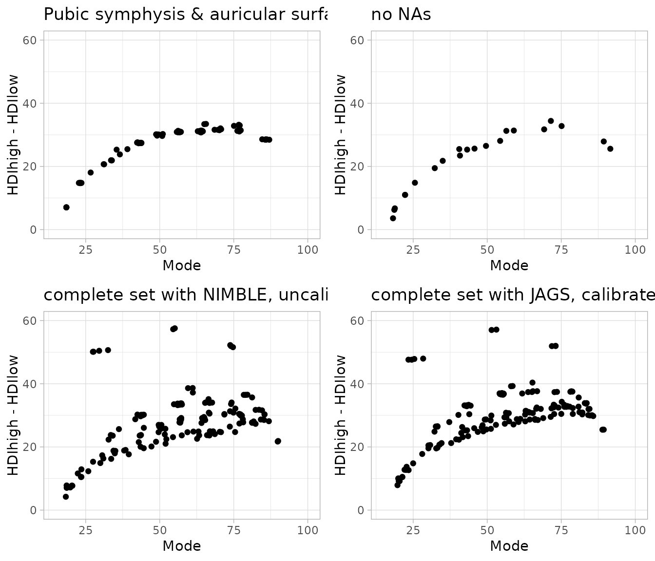
As noted previously (Müller-Scheeßel et al. 2026), the HDI ranges are lowest in early life and increase from there onwards. However, at about an age mode of 60–70 years, they start to shrink again.

The plots of the joined analysis of the auricular surface and the pubic symphysis as well as that for the data set without NAs look very similar, despite the fact that the first model contained much more entries than the second. In both cases, the point estimates form a rather clean arc. In contrast, the complete model looks rather messy with some extreme outliers, presumably from individuals were only the weakest method, dental wear, was assessable. Furthermore, the clean arc of the first two models has disappeared because middle-aged individuals were assessed overall younger than in the first two models. In comparison, the complete model with the calibration term of 5 years has again moved closer to the model without NAs. This we would take as a hint that the estimates of the model with calibration term are more conservative.

Next, we compare the calibrated estimated ages-at-death with the true ages-at-death known for 16 individuals.

chelsea_complete$estimated_age <- 
  round(chelsea_complete_cal_diag_red_ages[,5],1)
chelsea_complete[,c("AGE", "known_age", "estimated_age")] |> 
  na.omit() |> knitr::kable()

	AGE	known_age	estimated_age
5	ADULT >46 YEARS	60	58.9
16	ADULT >46 YEARS	67	75.2
24	ADULT 36-45 YEARS	44	56.5
62	ADULT 36-45 YEARS	61	58.6
76	ADULT >46 YEARS	70	78.1
93	ADULT >46 YEARS	84	71.8
100	ADULT >46 YEARS	66	62.8
103	ADULT >46 YEARS	84	80.8
105	ADULT >46 YEARS	78	85.8
107	ADULT >46 YEARS	68	78.8
109	ADULT >46 YEARS	56	66.7
114	ADULT 36-45 YEARS	70	48.4
122	ADULT >46 YEARS	68	66.5
143	ADULT >46 YEARS	54	56.2
144	ADULT 26-35 YEARS	32	32.6
161	ADULT 36-45 YEARS	70	55.6

The agreement between known and estimated age-at-death is already very satisfying. Eye-balling shows only three more severe outliers (nos. 24, 114 and 161). The traditional aging method is wrong in three cases (nos. 62, 114, 161). For a more systematic comparison, we evoke the helper function age.comp.summary().

summary_list <- lapply(c("Mode", "Median", "Mean"), function(choice) {
  age.comp.summary(mcmc_list = chelsea_complete_cal_res, 
                   known_age = chelsea_complete$known_age,
            age_identifier = "age.s_c",
                   mean_choice = choice)})
summary_mat <- do.call(rbind, summary_list)
rownames(summary_mat) <- c("Mode", "Median", "Mean")
summary_mat |> t() |> knitr::kable(digits = 2)

	Mode	Median	Mean
Bias	0.09	0.44	0.52
corrPearson	0.74	0.75	0.74
corr_p	0.00	0.00	0.00
Residual_slope	0.25	0.25	0.27
Inaccuracy	7.52	7.31	7.30
RMSE	9.47	9.35	9.36
TMNLP	3.99	3.99	3.99
CRPS	5.26	5.26	5.26

Above the resulting coverage for 95% credibility was computed. As already pointed out above, the first six frequentist quality measures are dependent on the point estimate and therefore malleable to the chosen measure of the mean. The mode is best in terms of the first four quality measures while the arithmetic mean performs better for Inaccuracy and RMSE. The median is somehow in-between. The two Bayesian measures TMNLP and CRPS, in contrast, do not change, regardless which point estimate was chosen.

When reviewing the quality measures itself (see Müller-Scheeßel et al. 2026 for a short review of some tests of age estimation methods), the performance is quite good. Most single methods will not reach an Inaccuracy of 7.3 years or a CRPS of 5.25.

A formal test of the coverage is the binomial test which checks if the resulting numbers deviate significantly from expectation. Below, we do this for several credibility ranges. Due to the small sample size of only 16 age-known individuals, we cannot expect any significant result.

sequential.binom.test(chelsea_complete_cal_res,
                      HDImass = c(seq(0.5, 0.9, 0.1), 0.95),
                      age_identifier = "age.s_c",
                      known_age = chelsea_complete$known_age) |> 
  knitr::kable(digits = 3)

coverage	n_in	perc	CI_low	CI_up	p_value
0.50	7	0.438	0.198	0.701	0.804
0.60	9	0.562	0.299	0.802	0.802
0.70	12	0.750	0.476	0.927	0.790
0.80	13	0.812	0.544	0.960	1.000
0.90	15	0.938	0.698	0.998	1.000
0.95	15	0.938	0.698	0.998	0.560

We show the relationship between known and estimated age-at-death also in a series of plots which are generated with the helper function age.comp.plot().

age.comp.plot(x = chelsea_complete_cal_diag,
            age_identifier = "age.s_c",
            known_age = chelsea_complete$known_age,
            mean_choice = "Mode")
#> Warning: Removed 25 rows containing missing values or values outside the scale range
#> (`geom_line()`).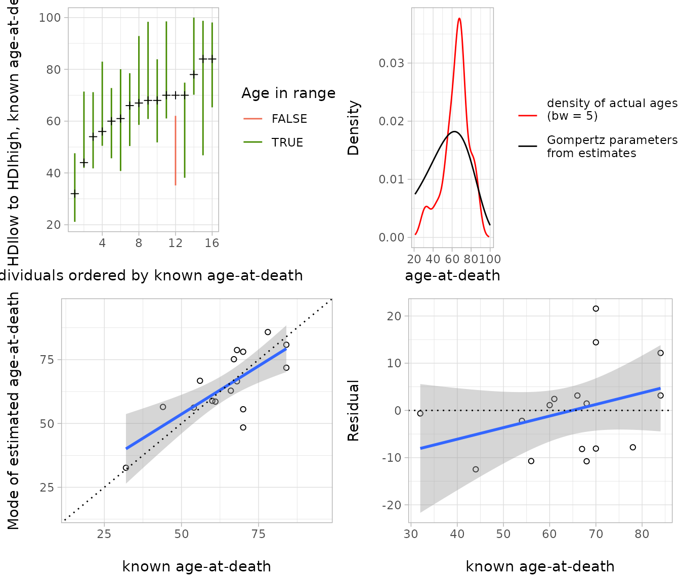

Only one HDI range does not include the true age (left top). The top right plot shows the Gompertz function based on the estimates of all individuals (in black) with the density of the known ages-at-death (in red). That the latter represent a part of the population seems from this plot at least not implausible. The two bottom plots illustrate the differences of the point estimate from the known age-at-death. Especially the right bottom plot also shows the systematic deviation which leads to a residual slope of 0.21. Most differences between estimated and known age are at about 10 years or below but one case deviates by more than 20 year.

Conclusions

One of the main aims of the above workflow was to show how the highest density intervals can be calibrated when several traits are observed but the data is incomplete. This entails to run a multivariate normal model with only those cases that do not contain any NA values and then set the calibration in such a way that the ensuing HDIs emulate that from the model with no NAs. For the Chelsea ‘Old church’ data set, this had lead to age ranges that fit to the known ages-at-death.

Apart from this, two further aspects which become apparent with the Chelsea ‘Old church’ data set merit attention. The first concerns the different mean and modal ages for the different model based on different traits and trait combinations. It has to be kept in mind that the ensuing samples are not identical and only partly overlap. That means that the different mean ages might well reflect true differences in the age composition of the respective samples. Especially in the case of the model of no NAs, that is the one where all traits were assessable, the low mean age is noteworthy, despite the fact that the plot with the ages and the HDIs looked very similar to the one with auricular surface and pubic symphsis. Therefore, we have to consider that age-at-death and completeness of trait observations is very probably not independent from one another. This suggests that missingness is not random with respect to age, which may bias multivariate estimates.

The second aspects relates to the highest density intervals: For the multivariate normal models, these were around 30 years of age. This is the same range which was found for the DRNNAGE system (Müller-Scheeßel et al. 2026) but also for the new ABDOU transition analysis (manuscript in prep.). It seems quite possible that with methods based on pathological changes in the skeleton, as those age markers essentially are (Fuchs et al. 2026), we cannot get below this threshold of 30 years. This seems to equal an inaccuracy level of about 6–7 years or a CRPS of about 4–5 years.

References

Cowie, Robert, Jelena Bekvalac, and Tania Kausmally. 2008. Late 17th- to 19th-century burial and earlier occupation at All Saints, Chelsea Old Church, Royal Borough of Kensington and Chelsea. Vol. 18. MoLAS Archaeology Studies Series. Museum of London Archaeology Service.

Fuchs, Katharina, Jo Appleby, Marie Louise Schjellerup Jørkov, et al. 2026. “Age-Related Disease or Disease-Related Age? Perspectives for Paleopathological Research.” International Journal of Paleopathology 53: 1–11. https://doi.org/https://doi.org/10.1016/j.ijpp.2026.02.003.

Kruschke, John K. 2015. Doing Bayesian data analysis: a tutorial with R, JAGS, and Stan. Academic Press.

Lovejoy, C. Owen, Richard S. Meindl, Robert G. Tague, and Bruce Latimer. 1997. “The comparative senescent biology of the hominoid pelvis and its implications for the use of age-at-death indicators in the human skeleton.” In Integrating archaeological demography: Multidisciplinary approaches to prehistoric population, vol. 24. Center for Archaeological Investigations Occasional Paper. Center for Archaeological Investigations.

Müller-Scheeßel, Nils, Christoph Rinne, and Katharina Fuchs. 2026. “A Fully Bayesian Approach to Adult Skeletal Age Estimation: Multivariate Latent Trait Modeling with Markov Chain Monte Carlo Sampling.” American Journal of Biological Anthropology.