To show how the age estimations of baytaAAR can be
compared with known age-at-death, we use the data set of Spitalfields
(Buckberry and Chamberlain 2002). The
individuals come from a crypt at Christ Church in Spitalfields, London
and were identified in terms of age and sex by plates on their coffins.
The following table gives an impression of the data:
data(spitalfields, package = "baytaAAR")
head(spitalfields)
#>   Age TO ST MI MA AP Sex
#> 1  16  1  1  1  1  2   F
#> 2  17  2  1  1  1  1   F
#> 3  19  1  2  1  1  1   F
#> 4  23  3  2  2  1  2   F
#> 5  27  1  1  3  1  1   F
#> 6  27  2  2  2  1  1   F
Buckberry and Chamberlain introduced a new scoring system of the pubic symphysis and thereby replaced a single score with multiple levels to several traits with fewer levels each.
For running the model, we use NIMBLE and the multivariate normal
likelihood (mnorm). In a real-life setting,
multicore should be set to TRUE to reduce
computation time. Still, even on modern hardware, the model will run for
up to several weeks until the usual quality criteria are met. However,
already a shorter run demonstrates the principle (for the full run see the results in Müller-Scheeßel et
al. 2026).
spitalfields_res <- bay.ta(
  framework = "NIMBLE",
  algorithm = "mnorm",
  multicore = F,
  method = spitalfields[,c(2:6)],
  minimum_age = 16,
  parameters = c("b", "a", "beta0", "beta", "thresh", "age.s", "Ustar"),
  thinSteps = 200,
  numSavedSteps = 500,
  seed = 331
)
For the sake of illustration, we skip the diagnostic checks here and
move directly to the comparison with known ages-at-death. For this,
baytaAAR provides several custom functions which
essentially work as wrappers around other R functions for
convenience.
As the name suggests, the function age.comp.summary()
summarizes standard quality measures of the comparison of known and
estimated ages-at-death. These fall into two groups:
- Frequentist point estimates
-
Bias- Arithmetic mean of the difference between known and estimated age of all individuals in the sample. -
corrPearson– Correlation between known and estimated age with -
p_value– p-value of that correlation and -
Residual_slope– Slope of the regression of the difference between known and estimated age. -
Inaccuracy– Arithmetic mean of the absolute difference between known and estimated age. -
RMSE– Root mean square error of known and estimated age.
- Bayesian density estimates
-
TMNLP– Test mean log posterior, a local evaluation of the probability density at the point of known age (Stull et al. 2022). -
CRPS– Continuous ranked probability score, a global evaluation of the probability density at the point of known age (Gneiting et al. 2007).
For nearly all measures, lower is better. The only exception is
corrPearson where larger is better. Because the differences
are squared with the RMSE, outliers influence this measure
more strongly than this is the case for Inaccuracy, and
therefore, the former tends to be higher than the latter. A similar
relationship exists between CRPS and TMNLP.
Overall, Müller-Scheeßel et al. found that the CRPS seems
to be more informative than the TMNLP and, therefore, the
CRPS is probably the most informative and single best
measure to compare the results between different age estimation methods
in terms of their quality to ‘predict’ age-at-death.
age.comp.summary() assumes that you choose one of the
point estimates Mode, Median,
Mean but in the code snippet below we demonstrate how all
three measures can be computed and tabulated in one go.
age.comp.summary() expects the raw output from
bay.ta() as well as a vector of known age-at-death. The
latter may contain NAs, these are subsequently simply
ignored.
summary_list <- lapply(c("Mode", "Median", "Mean"), function(choice) {
  age.comp.summary(mcmc_list = spitalfields_res,
                   known_age = spitalfields$Age,
                   mean_choice = choice)})
summary_mat <- do.call(rbind, summary_list)
rownames(summary_mat) <- c("Mode", "Median", "Mean")
summary_mat |> t() |> knitr::kable(digits = 2)| Mode | Median | Mean | |
|---|---|---|---|
| Bias | 2.64 | 4.33 | 5.42 |
| corrPearson | 0.63 | 0.67 | 0.67 |
| corr_p | 0.00 | 0.00 | 0.00 |
| Residual_slope | 0.31 | 0.39 | 0.47 |
| Inaccuracy | 12.52 | 11.21 | 11.19 |
| RMSE | 15.88 | 14.28 | 14.06 |
| TMNLP | 4.95 | 4.95 | 4.95 |
| CRPS | 8.03 | 8.03 | 8.03 |
As the above table shows, it can make quite a difference which mean
measures Mean (= arithmetic mean), Median or
Mode is chosen for the frequentist point estimate. In this
case, the differences are even exaggerated because there are not enough
iterations for stable estimates. On the other hand, the Bayesian
estimates are not influenced by the choice of the mean measure because
they are based on the probability density of the posterior.
Age estimation methods usually also supply minimum and maximum values
for their estimates, so a range within which the true age-at-death
should fall. Ideally, this range should adapt to the
credibility/confidence level chosen, and the percentage of the true
cases, the so-called coverage should be close to the chosen
level. To test coverage formally, in the literature the
cumulative binomial test has been proposed (Konigsberg et al. 2008). The wrapper
sequential.binom.test() calculates this test for several
given credibility levels:
sequential.binom.test(spitalfields_res,
                      HDImass = c(seq(0.5, 0.9, 0.1), 0.95),
                      known_age = spitalfields$Age) |>
knitr::kable(digits = 3)| coverage | n_in | perc | CI_low | CI_up | p_value |
|---|---|---|---|---|---|
| 0.50 | 80 | 0.444 | 0.371 | 0.520 | 0.157 |
| 0.60 | 99 | 0.550 | 0.474 | 0.624 | 0.172 |
| 0.70 | 122 | 0.678 | 0.604 | 0.745 | 0.516 |
| 0.80 | 137 | 0.761 | 0.692 | 0.821 | 0.192 |
| 0.90 | 158 | 0.878 | 0.821 | 0.922 | 0.319 |
| 0.95 | 166 | 0.922 | 0.873 | 0.957 | 0.088 |
In the table above, for all levels the confidence intervals of the observed coverage include the expected coverage. Thus, this result suggests that the model is able to ‘predict’ age-at-death with the correct level of confidence.
Finally, age.comp.plot() shows the relationship between
estimated and known ages-at-death graphically. Its four plots convey the
following information:
Top left: Comparison of estimated highest density intervals with known ages (green = age within HDI, red = age outside HDI, individuals ordered according to known age-at-death).
Top right: Comparison of the density of known ages with a Gompertz function derived from the arithmetic mean of the estimated population parameters and .
Bottom left: Scatter plot of known and estimated ages with regression line in blue. The dotted line marks perfect equivalence.
Bottom right: Slope of the regression line from the left bottom image (cf. goodness-of-fit measure
Residual_slopefrom the functionage.comp.summary()).
Again, it can make quite a difference which mean measure is chosen
for the point estimate for the two lower plots. The left top plot is not
affected because the highest density intervals derive from the
density distribution of the age estimates. For the right top plot, the
Gompertz parameters are always taken from the arithmetic mean because
only then the deterministic relationship between
and
holds. As the code below shows, age.comp.plot() expects the
output from diagnostic.summary() so the credibility level
chosen (HDImass) there also determines what is shown in the
top left plot. age.comp.plot() presupposes, of course, that
there is a vector with known ages.
diagnostic.summary(spitalfields_res, HDImass = 0.95) |>
  age.comp.plot(known_age = spitalfields$Age)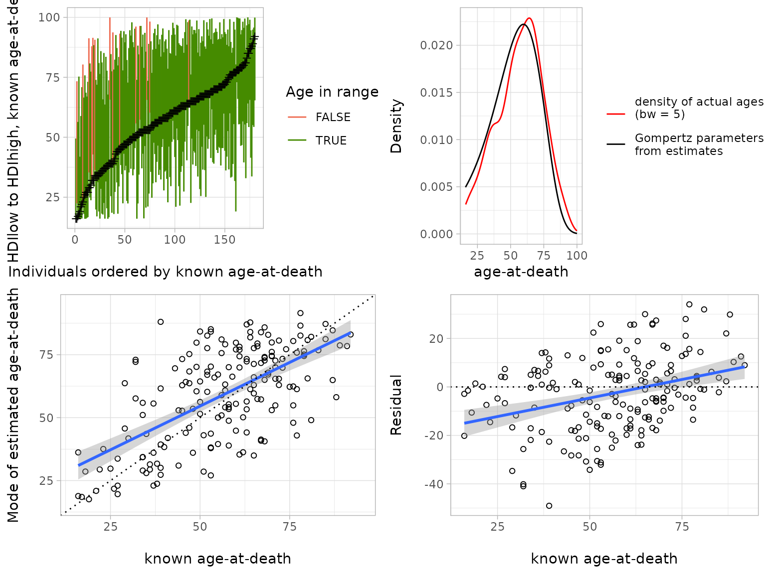
The top left plot visualizes the result of the bottom line of the
last table: Only eleven estimates, marked in red, do not contain the
true age-at-death at the default credibility level 0.95. The top right
plot illustrates the good agreement of the estimated Gompertz parameters
fed into a Gompertz function with the density of the true ages-at-death.
The bottom left plot is related to the correlation expressed in
corrPearson, of course. The bottom-right plot shows the
same relationship, relative to the dotted line in the bottom-left plot
which is equivalent to the zero-line on the bottom right. The regression
line in blue on the bottom right is nothing else than the quality
measure Residual_slope. This plot also visualizes the
spread of the difference between true and estimated age-at-death.