Mathematical background

Benjamin Gompertz and the Gompertz distribution

Central to baytaAAR is the Gompertz distribution, named after the British mathematician B. Gompertz (1779–1865) who first presented it in 1825 (Gompertz 1825).

Hazard, survival and the ensuing probability distribution are defined as follows (see also Wood et al. 2002, 146):

$$\begin{align} \mu(t) & = \alpha \cdot \exp(\beta t) \\ S(t) & = \exp\big(\frac{\alpha}{\beta} \cdot (1-\exp(\beta t))\big) \\ f_0(t \mid \alpha,\beta) & = \alpha \cdot \exp\big(\beta t + \frac{\alpha}{\beta} \cdot (1-\exp(\beta t))\big) \end{align}$$

Despite or even because of its simplicity, it is still widely applied. Instrumental for baytaAAR is the strong empirical correlation between its two parameters $\alpha$ and $\beta$, the so-called Strehler-Mildvan-correlation (Strehler and Mildvan 1960). This makes it possible to reformulate it as essentially a one-parameter distribution that still captures human mortality adequately. The empirical correlation between the two parameters at the age of 15 years was defined by T. Sasaki and O. Kondo (2016, 529 fig. 1) as follows:

$$\begin{align} Sab & = -2.624 \\ Sbb & = 0.0393 \\ Ma & = -7.119 \\ Mb & = 0.0718 \\ V & = 0.0823 \\ ln\alpha & \sim \mathrm{dnorm} (Sab \cdot (\beta - Mb)/Sbb + Ma, 1 / V ) \\ \alpha & = \exp(ln\alpha) \end{align}$$ Here, a normal distribution with a variance term of 0.0823 serves as a basis to model log-transformed $\alpha$. If the variance term is omitted, the relationship between $\alpha$ and $\beta$ becomes deterministic:

$$\alpha =\exp(Sab \cdot (\beta - Mb)/Sbb + Ma)$$ If the starting age is not 15, we simulate the relation with the internal function gomp.a0().

The parameter $\beta$ is estimated from the observed data, thereby defining the overall level of mortality of the respective population and the age range of the individuals. The following figure, taken from Müller-Scheeßel et al. (2024, 4 fig. 1), shows Gompertz hazard, survival and density curves with different $\beta$ values:

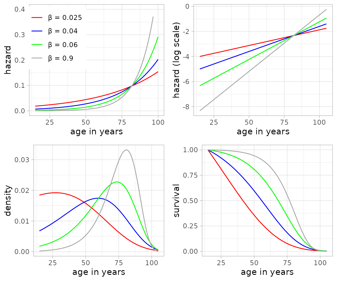
The modal age M derives naturally from the Gompertz model. It equals the peak of the curves in the lower left image. It is a useful parameter for adult mortality as it does not change with the starting observed age as life expectancy does (Missov et al. 2015). So, for example, e₂₀ (life expectancy from age 20) will differ from e₂₅ (life expectancy from age 25), and the one is not easily translated to the other. This is not the case with the modal age M. The modal age M is defined as: $$M = \frac{1}{\beta} \cdot log\big(\frac{\beta}{\alpha}\big)$$

The Gompertz distribution with NIMBLE and JAGS

The Gompertz distribution is implemented in NIMBLE and JAGS with the so-called ‘ones trick’, which is a simple, convenient way to implement custom distributions (Kruschke 2015, 214–15). Theoretically, NIMBLE allows custom functions to be added as nimble functions compiled at runtime but we wanted to make sure that the results of the two frameworks are as similar as possible.

Mathematical notation

Building on this mortality model, we now describe how it is embedded in the latent trait framework used by baytaAAR.

The observed data are written as $y_{i,j}$ where $i$ indexes individuals from 1 to $N$ and $j$ indexes traits (skeletal age “indicators”) from 1 to $J$. Because the data are recorded for ordinal categorical traits the values for each trait are positive integers. The number of states per trait is given as $K_j$. With $K_j$ states per trait $j$, there are $K_j - 1$ thresholds for each trait.

$$i = 1,\dots,N, \qquad j = 1,\dots,J, \qquad k = 1,\dots,K_j$$

As stated above, the Gompertz model has two parameters $\alpha$ and $\beta$. The prior for $\beta$ is:

$$\beta \sim \textit{U}(a = 0.02,\; b = 0.1)$$ where $U(a, b)$ denotes a uniform distribution with density 1/(b - a) between a and b. Simplifying the equation of Sasaki and Kondo above, $\alpha$ is given deterministically as:

$$\alpha = \exp(-66.77 \cdot \beta - 2.325)$$

The prior for individual ages $t_i$, where $t$ is the age-at-death, is

$$t_i \sim \textit{Gompertz}(\alpha,\; \beta)$$ The starting age $t_0$ is usually at 15 years, and the distribution is truncated at 100 years - starting age, reflecting a maximally expected life span of 100 years.

The thresholds within each trait are represented using the symbol $\gamma$, so that for a trait with five stages, the thresholds are $\gamma_{k_1 = 1} < \gamma_{k_1 = 2} < \gamma_{k_1 = 3} < \gamma_{k_1 = 4}$. To ensure identifiability, all $\gamma_{k_j = 1} = 1.5$.

The priors for thresholds with more than two states are:

$$\gamma_{k=2,…,K_j} \sim \textit{TN}( \mu = k + 0.5,\; \sigma = 10,\; a,\; b = \infty)$$

where $TN()$ is a truncated normal distribution with left truncation at a and right truncation at b. Because the thresholds must be ordered, for the JAGS-model, $a = 1.5$, and the simulated thresholds are sorted in ascending order. NIMBLE does not have a sort-function, so there $a = \gamma_{k-1}$.

For each individual there is a vector of latent traits $z_i$ of length $J$ (number of traits). For the simple probit model with conditional independence, the elements of these vectors are modeled separately with normal distributions:

$$z_{i,j} \sim \mathcal{N}(\mu_{i,j},\; \sigma = 1)$$

For identifiability, $\sigma$ is fixed at $unity$ (1).

For the complex probit model, these vectors follow a multivariate normal distribution:

$$\boldsymbol{z}_i \sim \mathcal{MVN}( {\mu}_{i,j},\; \mathbf{R})$$

We use a “flat” prior by Lewandowski, Kurowicka, & Joe (2009) for the correlation matrix:

$$\mathbf{R} \sim \textit{LKJ}(\eta = 1)$$

For $\eta = 1$, this prior is uniform over the space of correlation matrices.

The components of the vector $\mu_{i}$ are:

$$\mu_{i,j} = \textit{beta}_{0_j} + \textit{beta}_j \cdot \ln(t_i)$$

with the priors for the $beta_0$ and $beta$ parameters within each trait $j$ being:

$$\textit{beta}_{0_j} \sim \textit{TN}(\mu = 0,\; \sigma = 10,\; a = -\infty,\; b = 0)$$

$$\textit{beta}_{j} \sim \textit{TN}(\mu = 0,\; \sigma = 10,\; a = 0,\; b = \infty)$$

JAGS and NIMBLE both have the distribution dinterval which is difficult to express succinctly:

$$y_{i,j} = \begin{cases} 1, & \text{if } z_{i,j} \le 1.5, \\[6pt] k_j, & \text{if } \gamma_{j,k_j-1} < z_{i,j} \le \gamma_{j,k_j}, \quad k_j=2,\dots,K_j-1, \\[6pt] K_j, & \text{if } \gamma_{j,K_j-1} < z_{i,j} \end{cases}$$

Because dinterval indexes categories from zero instead of one, the observed trait levels and thresholds are internally shifted by one unit.

The proper initialization of the chains is crucial in probit regression. Each chain starts with different parameter values to enhance mixing, and most parameters are initialized with random values from uniform distributions. For Gompertz $\beta$ initial values are drawn from 0.02–0.1, for $beta$ the range is 0.5–1, and for $beta_0$–10––3. The init value for age $t_i$ is 20–40. To this value, the starting value (15 by default) is added. The correlation matrix is for all chains initialized with an identity matrix (ones on the diagonal and zeros elsewhere). The thresholds are initialized with k + 0.5 and the vector of latent traits $z_i$ with $y_{i,j} - \textit{U}(-0.2, 0.2)$.

---

References

Gompertz, Benjamin. 1825. “On the Nature of the Function Expressive of the Law of Human Mortality, and on a New Mode of Determining the Value of Life Contingencies.” Philosophical Transactions of the Royal Society of London 115: 513–83. https://doi.org/10.1098/rstl.1825.0026.

Kruschke, John K. 2015. Doing Bayesian data analysis: a tutorial with R, JAGS, and Stan. Academic Press.

Lewandowski, Daniel, Dorota Kurowicka, and Harry Joe. 2009. “Generating random correlation matrices based on vines and extended onion method.” Journal of Multivariate Analysis 100 (9): 1989–2001. https://doi.org/10.1016/j.jmva.2009.04.008.

Missov, Trifon I., Adam Lenart, Laszlo Nemeth, Vladimir Canudas-Romo, and James W. Vaupel. 2015. “The Gompertz Force of Mortality in Terms of the Modal Age at Death.” Demographic Research 32: 1031–48.

Müller-Scheeßel, Nils, Christoph Rinne, and Katharina Fuchs. 2024. “Adult mortality in the metropolis of London 1100–1850: A Bayesian view based on osteological data.” American Journal of Biological Anthropology 185 (3): e25025. https://doi.org/10.1002/ajpa.25025.

Sasaki, Tomohiko, and Osamu Kondo. 2016. “An Informative Prior Probability Distribution of the Gompertz Parameters for Bayesian Approaches in Paleodemography.” American Journal of Physical Anthropology 159 (3): 523–33.

Strehler, Bernard L., and Albert S. Mildvan. 1960. “General Theory of Mortality and Aging.” Science 132 (3418): 14–21.

Wood, James W., Darryl J. Holman, Kathleen A. O’Connor, and Rebecca J. Ferrell. 2002. “Mortality Models for Paleodemography.” In Paleodemography: Age Distributions from Skeletal Samples, edited by Robert D. Hoppa and James W. Vaupel. Cambridge University Press.