Life table correction • mortAAR

Load libraries

library(mortAAR)
library(magrittr)

Smoothing of data

Due to the nature of most anthropological age estimation methods, life tables from archaeological series often contain artificial jumps in the data. To counteract this effect, mortAAR provides the option to interpolate values for adults by a monotonic cubic spline. Usual options are ‘10’, ‘15’ or ‘20’ which will interpolate the values for individuals aged 20 or older by 10-, 15- or 20-year cumulated values. This option should be used with caution, as diagnostic features of the life table may be smoothed out or lost. This option is only available when the Standard or Equal5 methods are used in prep.life.table.

As an example, we use data from the Early Neolithic cemetery of Nitra. First, we prepare the data, calculate the life table and plot d_x- and q_x-curves. The age-classes 25–44 show a bimodal distribution which appears unrealistic. Furthermore, the curve sharply drops after 40 which also looks very unnatural.

nitra_prep <- prep.life.table(nitra, method="Equal5", 
                              agebeg = "age_start", ageend = "age_end")
nitra_life <- life.table(nitra_prep)
plot(nitra_life, display=c("dx","qx"))

## $dx

## 
## $qx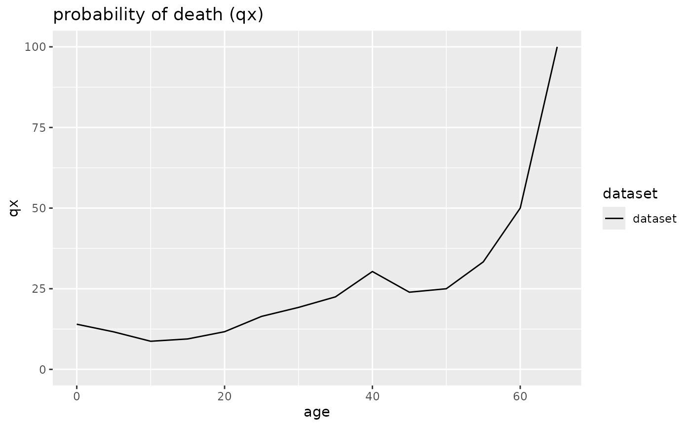

Next we test how the plot changes when the spline option is set to 10 or 20 years. In both cases, the smoothing is only applied to the age groups 20 and above.

nitra_life <- life.table(nitra_prep,option_spline = 10)
plot(nitra_life, display=c("dx","qx"))

## $dx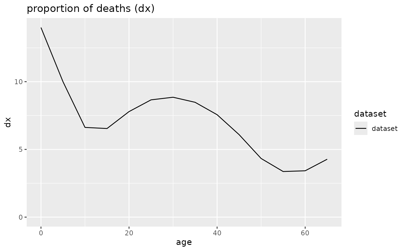

## 
## $qx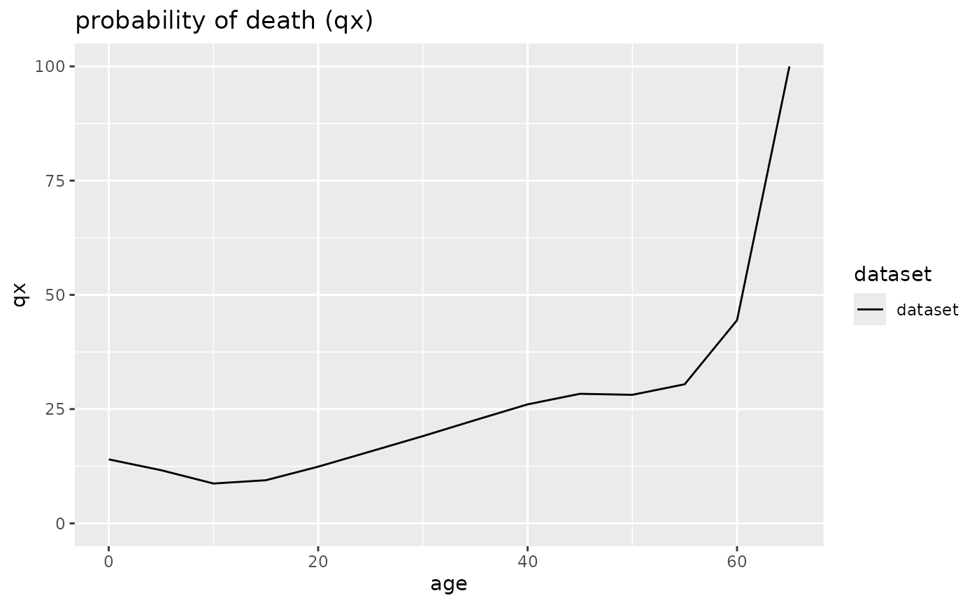

nitra_life <- life.table(nitra_prep,option_spline = 20)
plot(nitra_life, display=c("dx","qx"))

## $dx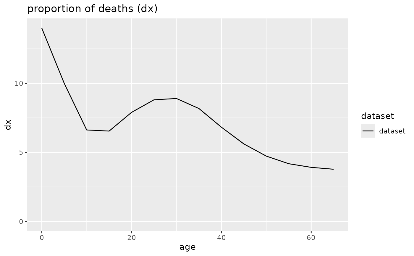

## 
## $qx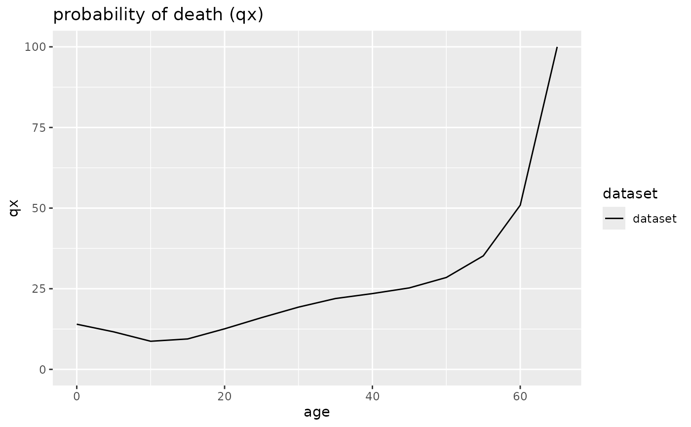

As expected, this produces much smoother curves. However, for the 10-year-option, the oldest age group shows a local maximum which is not reflected in the original data and therefore is an artefact of the smoothing algorithm working on the available data. In this case, the 20-year-option seems to offer a better compromise between a much more natural looking curve and still fidelity to the original data.

Representativeness of data

Anthropological data from archaeological contexts are necessarily fragmentary. The question is whether this fragmentation leads to completely unreliable inferences when statistical methods are applied to it. K. M. Weiss (1973, 46f.) and C. Masset and J.-P. Bocquet-Appel (1977; see also Herrmann et al. 1990, 306f.) have therefore devised indices which assess whether non-adult age groups are represented in proportions as expected based on comparable modern data. Whether this is really applicable to archaeological data-sets is a matter of debate.

Weiss chose the mortality (q_x) as the deciding factor and claimed that (1) the probability of death of the age group 10-15 (₅q₁₀) should be lower than that of the group 15-20 (₅q₁₅) and that (2) the latter in turn should be lower than that of age group 0-5 (₅q₀).

In contrast, Bocquet-Appel and Masset took the raw number of dead (D_x) and asserted that (1) the ratio of individuals who died between 5 and 10 (D_5-10) and those who died between 10 and 15 years (D_10-15) should be equal or larger than 2 and that (2) the ratio of those having died between 5 and 15 (D_5-15) and all adults (>= 20; D₂₀₊) should be at least 0.1.

If either condition is not met, the results from such data should be treated with extreme caution as the mortality structure is different from that of known populations. Because of the structure of these indices, they only give meaningful results if 5-year-age categories have been chosen for the non-adults.

Recently, B. Taylor and M. Oxenham (2024) added a comparison of Total fertility rates (TRF) according to different formulas which depend either on subadults or adults. The formulas Taylor and Oxenham used either weight all individuals aged 0–14 against all individuals or all individuals aged 15–49 against all individuals aged 15+. The formulas differ from the original ones published by C. McFadden and M. Oxenham (2018) and B. Taylor et al. (2023) because the data basis is sightly different. If the results of the formulas deviate by more than 0.692 (the standard error of estimate, SEE), they conclude that this indicates a problem with the age structure. In contrast to the tests by Weiss and Masset and Bocquet-Appel, there is no need to divide the sample into 5-year-steps, as long as the limits at 15 and 50 years are respected.

As an example, we use the data-set of the medieval cemetery of Schleswig.

schleswig <- life.table(schleswig_ma[c("a", "Dx")])
lt.representativity(schleswig)

##     approach            condition value1 value2 result outcome
## 1   weiss_i1           5q0 > 5q15  20.24   4.91   4.12    TRUE
## 2   weiss_i2          5q10 < 5q15   6.86   4.91   1.40   FALSE
## 3    child_i    (5D5 / 5D10) >= 2  22.00  12.00   1.83   FALSE
## 4 juvenile_i (10D5 / D20+) >= 0.1  34.00 155.00   0.22    TRUE
## 5        TFR       TFR_SA = TFR_A   4.83   6.99   2.16   FALSE

The result is a data frame where the individual conditions with the actual results are listed. The last column indicates whether each condition is met or not. In the case of the Schleswig cemetery, only the Weiss criterium (1) and the Bocquet-Appel/Masset criterium (2) is TRUE, the other three are FALSE. Therefore, it can be argued that the Schleswig data is not representative of a complete once-living population. However, it might be that the Bocquet-Appel/Masset criterium (1) is too conservative as only two additional individuals would have to have died at this age to bring the ratio above 2 (Herrmann et al. 1990, 307). P. Sellier (1989, 23) has even argued that the ratio should be 1.5 instead of 2. In this case, both criteria of Bocquet-Appel and Masset would be met for the Schleswig cemetery.

Correction of life table data after Bocquet-Appel and Masset

It is generally assumed that most skeletal populations lack the youngest age group. Life tables resulting from such populations will be misleading as they suggest that the mortality of younger children was lower than it actually was and that life expectancy was higher. For correcting these missing individuals, Masset and Bocquet-Appel (1977; see also Herrmann et al. 1990, 307) developed several calculations based on regression analyses of modern comparable mortality data. Although these recommendations are more than 40 years old, they still surface in text books (e. g. Grupe et al. 2015, 418–19). However, the applicability of these indices to archaeological data is debatable and does not necessarily lead to reliable results. Therefore, the correction must be applied with caution and ideally only after assessing the representativeness of the base data with the function lt.representativity.

The equations conceived by Masset and Bocquet-Appel are relatively complex. Life expectancy at the time of birth is computed as follows:

$e^0_x = 78.721 * log_{10} \sqrt{\frac{D_{20+}}{ D_{5-14}}} - 3.384 \pm 1.503$

The equation approaches 75 years of life expectancy when there is a ratio of adults to 5–14-year old of 100 to 1 as the term $log_{10} \sqrt{\frac{D_{20+}}{ D_{5-14}}})$ will then tend towards 1. Higher proportions of non-adults will likewise lead to lower life expectancy values.

The probability of death in the first and the first five years is similarly constructed:

$_1q_0 = 0.568 * \sqrt{log_{10}(\frac{200*D_{5-14}}{D_{20+}}}) - 0.438 \pm 0.016$

$_5q_0 = 1.154 * \sqrt{log_{10}(\frac{200*D_{5-14}}{D_{20+}}}) - 1.014 \pm 0.041$

The corrected Schleswig data¹ are as follows:

schleswig <- life.table(schleswig_ma[c("a", "Dx")])
lt.correction(schleswig)

## $indices
##   method  value range_start range_end
## 1     e0 22.549      21.046    24.052
## 2    1q0  0.290       0.274     0.306
## 3    5q0  0.465       0.424     0.506
## 
## $life_table_corr
## 
##   mortAAR life table (n = 368.1 individuals)
## 
## Life expectancy at birth (e0): 21.129
## 
##         x a    Ax      Dx     dx      lx      qx      Lx       Tx     ex
## 1    0--4 5 1.667 171.102 46.482 100.000  46.482 345.059 2112.914 21.129
## 2    5--9 5 2.500  22.000  5.977  53.518  11.168 252.648 1767.854 33.033
## 3  10--14 5 2.500  12.000  3.260  47.541   6.857 229.556 1515.207 31.871
## 4  15--19 5 2.500   8.000  2.173  44.281   4.908 215.973 1285.650 29.034
## 5  20--26 7 3.500  15.000  4.075  42.108   9.677 280.493 1069.677 25.403
## 6  27--33 7 3.500  30.000  8.150  38.033  21.429 237.706  789.184 20.750
## 7  34--40 7 3.500  12.000  3.260  29.883  10.909 197.771  551.478 18.455
## 8  41--47 7 3.500  19.000  5.162  26.623  19.388 168.296  353.707 13.286
## 9  48--54 7 3.500  36.000  9.780  21.461  45.570 116.001  185.411  8.639
## 10 55--61 7 3.500  28.000  7.607  11.682  65.116  55.148   69.410  5.942
## 11 62--68 7 3.500  15.000  4.075   4.075 100.000  14.262   14.262  3.500
##    rel_popx
## 1    16.331
## 2    11.957
## 3    10.864
## 4    10.222
## 5    13.275
## 6    11.250
## 7     9.360
## 8     7.965
## 9     5.490
## 10    2.610
## 11    0.675

Apart from the corrected life table, it also lists – as separate data.frame – the indices ( $e^0$ , $_1q_0$ and $_5q_0$ ) computed by the formulas of Masset and Bocquet-Appel. Compare this to the uncorrected values:

life.table(schleswig_ma[c("a", "Dx")])

## 
##   mortAAR life table (n = 247 individuals)
## 
## Life expectancy at birth (e0): 30.671
## 
##         x a    Ax Dx     dx      lx      qx      Lx       Tx     ex rel_popx
## 1    0--4 5 1.667 50 20.243 100.000  20.243 432.524 3067.139 30.671   14.102
## 2    5--9 5 2.500 22  8.907  79.757  11.168 376.518 2634.615 33.033   12.276
## 3  10--14 5 2.500 12  4.858  70.850   6.857 342.105 2258.097 31.871   11.154
## 4  15--19 5 2.500  8  3.239  65.992   4.908 321.862 1915.992 29.034   10.494
## 5  20--26 7 3.500 15  6.073  62.753   9.677 418.016 1594.130 25.403   13.629
## 6  27--33 7 3.500 30 12.146  56.680  21.429 354.251 1176.113 20.750   11.550
## 7  34--40 7 3.500 12  4.858  44.534  10.909 294.737  821.862 18.455    9.610
## 8  41--47 7 3.500 19  7.692  39.676  19.388 250.810  527.126 13.286    8.177
## 9  48--54 7 3.500 36 14.575  31.984  45.570 172.874  276.316  8.639    5.636
## 10 55--61 7 3.500 28 11.336  17.409  65.116  82.186  103.441  5.942    2.680
## 11 62--68 7 3.500 15  6.073   6.073 100.000  21.255   21.255  3.500    0.693

With the uncorrected data, the youngest age group (years 0–4) accounts for only about 20% of the population. However, according to the formulas by Masset and Bocquet-Appel, this number should be more than doubled (46%). This implies that in reality nearly 50% of the individuals died before they reached age 5. Applying this value to the life table, the number of individuals increases from 247 to 368 and at the same time the life expectancy at birth decreases from 30.7 to 21.1 years. Please note that this value differs slightly from the value computed by the formula by Masset and Bocquet-Appel (22.5 years). This can be explained by the fact that the life expectancy of the life table includes all individuals. However, the value of 21.1 years is still in the range of 21.0 to 24.1 years (see indices) given by Masset and Bocquet-Appel.

lt.representativity(lt.correction(schleswig)$life_table_corr)

##     approach            condition value1 value2 result outcome
## 1   weiss_i1           5q0 > 5q15  46.48   4.91   9.47    TRUE
## 2   weiss_i2          5q10 < 5q15   6.86   4.91   1.40   FALSE
## 3    child_i    (5D5 / 5D10) >= 2  22.00  12.00   1.83   FALSE
## 4 juvenile_i (10D5 / D20+) >= 0.1  34.00 155.00   0.22    TRUE
## 5        TFR       TFR_SA = TFR_A   6.40   6.99   0.60    TRUE

Because the correction only applies to the youngest age group, it has no effect on the tests for representativeness by Weiss and Masset and Bocquet-Appel. The correction, however, affects the test by Taylor et al. After correction, the Total fertility rate based on the subadult index is much closer to the value computed from the individuals aged 15 and above. As the difference is below 0.692, the test now would not suspect a biased population. This might be taken as hint that the ‘true’ TFR-value is closer to 7 than to 4 and that the correction by Masset and Bocquet-Appel was both necessary and produced reasonable estimates.

References

Grupe, Gisela, Michaela Harbeck, and George C. McGlynn. 2015. Prähistorische Anthropologie. Springer.

Herrmann, B., G. Grupe, S. Hummel, H. Piepenbrink, and H. Schutkowski. 1990. Praehistorische Anthropologie: Leitfaden Der Feld- Und Labormethoden. Springer.

Masset, Claude, and Jean-Pierre Bocquet. 1977. “Estimateurs En Paléodémographie.” L’Homme 17 (4): 65–90.

McFadden, Clare, and Marc F. Oxenham. 2018. “The D0-14/D ratio: A new paleodemographic index and equation for estimating total fertility rates.” American Journal of Physical Anthropology 165 (3): 471–79.

Sellier, Pascal. 1989. “Hypotheses and Estimators for the Demographic Interpretation of the Chalcolithic Population from Mehrgarh, Pakistan.” East and West 39 (1/4): 11–42.

Taylor, B. R., M. Oxenham, and C. McFadden. 2023. “Estimating fertility using adults: A method for under-enumerated pre-adult skeletal samples.” American Journal of Biological Anthropology 181 (2): 262–70. https://doi.org/10.1002/ajpa.24739.

Taylor, Bonnie R., and Marc F. Oxenham. 2024. “A method for detecting bias in human archaeological cemetery samples.” International Journal of Osteoarchaeology, 0. https://doi.org/10.1002/oa.3379.

Weiss, Kenneth M., and H. Martin Wobst. 1973. “Demographic Models for Anthropology.” Memoirs of the Society for American Archaeology 27: i–186.